記述統計量

Greg Nishihara

2024 / 07 / 07

Mean and expectation

Mean, average (平均値) or Expectation（期待値）

Add all values \((x_i)\) and divide by the total number of samples \((i)\). The population mean is \(\mu\) and the sample mean is \(\overline{X}\).

\[ \mu \equiv \overline{X} = \frac{1}{n} \sum_{i=1}^{n} x_i \] \[ \text{平均値} = \frac{\text{資料の変量の総和}}{\text{資料の個数}} \]

Deviation, residual

• Deviation: 偏差
• Residual: 残渣

Data: x = {12, 19, 3, 8, 9, 10, 16, 9, 13, 7}

Mean or average

mean(x)

[1] 10.6

Deviation or residual

x - mean(x)

 [1]  1.4  8.4 -7.6 -2.6 -1.6 -0.6  5.4 -1.6  2.4 -3.6

Linearity of the expectation（線形性）

\(a\) is a constant (定数) and \(X\) is the random variable (確率変数).

\[ E[aX] = aE[X] \]

• \(X\): x = {12, 19, 3, 8, 9, 10, 16, 9, 13, 7}
• \(aX = 5X\): ax = 5 × {12, 19, 3, 8, 9, 10, 16, 9, 13, 7} = {90, 55, 20, 90, 55, 10, 30, 30, 40, 70}

Linearity of the expectation（線形性）

Multiplying a random variable by a constant shifts the mean of the random variable by the same magnitude (constant).

\[ E[aX] = aE[X] \]

mean(x)

[1] 10.6

5 * mean(x)

[1] 53

mean(5 * x)

[1] 53

Monotonicity (単調性)

\[ X \leq Y \rightarrow E[X] \leq E[Y] \]

• x = {2,5,4}

• y = {9,7,9}

• 3.6666667 ≤ 8.3333333

Non-multiplicativity (非乗法性)

If the random variables \(X\) and \(Y\) are not independent (非独立性) of each other,

\[ E[XY] \neq E[X]\cdot E[Y] \]

mean(x * y)

[1] 210.6681

mean(x) * mean(y)

[1] 206.8307

Non-multiplicativity (非乗法性)

If the random variables are independent (独立性) of each other,

\[ E[XY] = E[X]\cdot E[Y] \]

mean(x * y)

[1] 199.3228

mean(x) * mean(y)

[1] 199.2973

Variance (分散)

The variance (分散) is the square of the difference of the random variable and \(E[X]\).

\[ \sigma^2\equiv Var(X) = E[(X - E[X])^2] = E[X^2] - E[X]^2 \]

It is a measure of scale (スケール) and decribes the amount of scatter in the data.

Variance（分散）

\[ \sigma^2\equiv Var(X) = E[(\underbrace{X - E[X]}_{\text{deviation}})^2] = E[X^2] - E[X]^2 \]

Properties of the variance（分散の一般的な性質）

Variance of a constant (定数) is zero

\[ Var(a) = 0 \]

Scale invariance (スケール普遍性)

\[ Var(aX+b) = a^2Var(X) \]

Additivity of independent variables（独立な確立変数の和の分散）

\[ Var(X+Y) = Var(X) + Var(Y) \]

Population variance (母分散)

When the population mean \((\mu)\) is known, then the population variance (\(\sigma^2\), 母分散) is

\[ \sigma^2 = \frac{1}{n}\sum_{i=1}^n\left(x_i - \mu\right)^2 \] However, we usually do not know the population mean. So, we must calculate the sample variance (標本分散).

Sample variance and the unbiased sample variance)

There are two ways to calculate the sample variance.

Sample variance (標本分散)

\[ \widehat{\sigma}^2=\frac{1}{n}\sum_{i=1}^n\left(x_i - \overline{x}\right)^2 \] The value of the sample variance \((\widehat{\sigma}^2)\) is smaller than the population variance (母分散). In otherwords, if \(n\) is small, then \(\widehat{\sigma}^2 \ll \sigma^2\).

Unbiased sample variance (不偏標本分散)

\[ s^2=\frac{1}{n-1}\sum_{i=1}^n\left(x_i - \overline{x}\right)^2 \] When \(n\) is small, use the unbiased sample variance (不偏標本分散 \((s^2)\)).

Unbiased sample variance (不偏標本分散)

• x = {4, 6, 2, 9, 3}
• mean: 4.8
• deviation: x = {-0.8, 1.2, -2.8, 4.2, -1.8}
• n: 5

z = x -  mean(x)
n = length(z)
sum(z^2) / (n - 1) # 数式で求めた値

[1] 7.7

var(x)             # Rの固有関数,必ず不遍分散を計算する

[1] 7.7

Variance is a measure of variation

\[ Var(aX+b) = a^2Var(X) \]

\[ \begin{aligned} Var(X) &= 1\\ Var(aX) &= 0.5\\ a^2Var(X) &= a^2 1 = 0.5\\ a &= \sqrt{0.5} = \frac{\sqrt{2}}{2}\\ \end{aligned} \]

Variance is a measure of variation

\[ Var(X+b) = Var(X) \]

\[ \begin{aligned} Var(X) &= 1\\ Var(X+b) &= 1\\ Var(X) &= Var(X+b) \end{aligned} \]

Standard deviation (標準偏差)

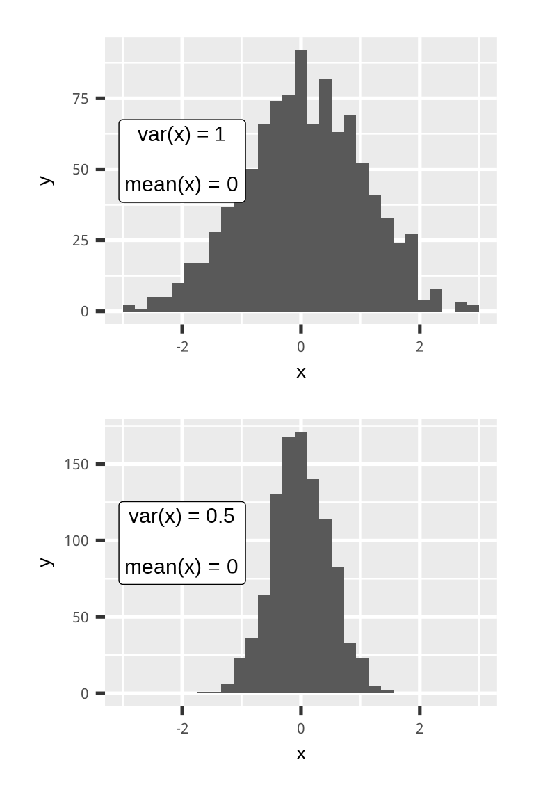
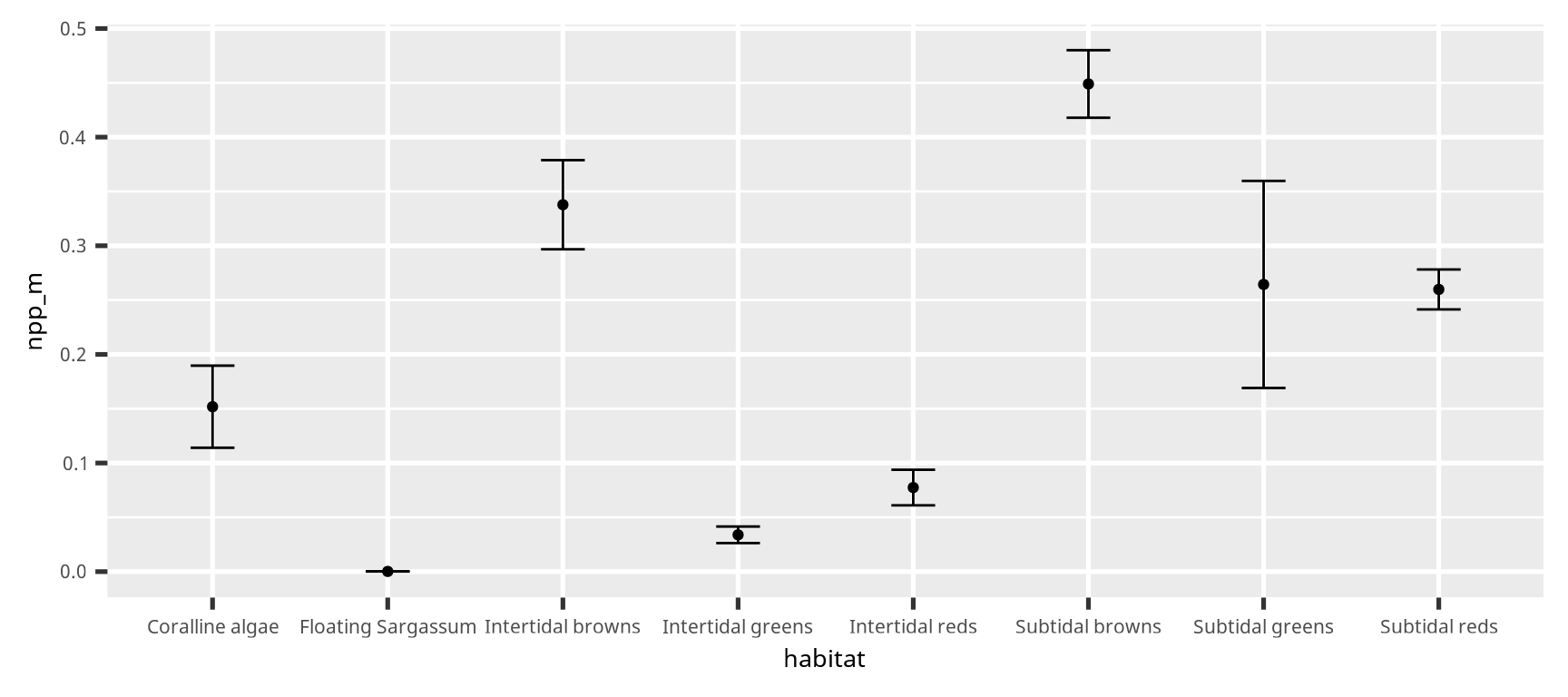
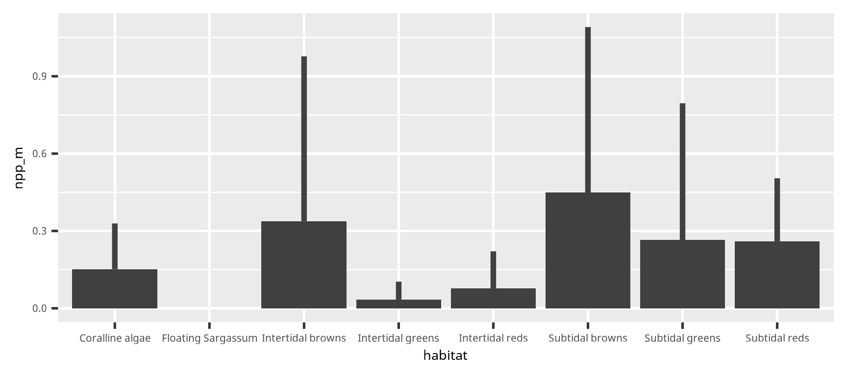
Variance (分散) describes how much the data is scattered around the expectation (mean). Since the sample variance is \(\sim\sum(x - \overline{x})^2\), it cannot be directly compared with the mean.

Standard deviation (標準偏差) (Std. Dev., S.D.)

\[ \sigma = \sqrt{\sigma^2} \equiv \sqrt{Var(X)} \]

The standard deviation is the positive root of the variance. Both variance and standard deviation describe the scatter of the data. Which variance to use? \(\widehat{\sigma}^2\) or \(s^2\)

Use the unbiased sample variance

\[ \text{Std. Dev.}=\sqrt{s^2}=\sqrt{\frac{1}{n-1}\sum_{i=1}^n (x_i -\overline{x})^2} \]

Standard error

The standard error (標準誤差) describes the precision of a statistic. All statistics have a standard error.

\[ S.E. = \frac{s}{\sqrt{n}} \] The S.E. decreases when sample size increase!

\[ \lim_{n\rightarrow\infty} \frac{s}{\sqrt{n}} = 0 \]

Median (中央値・メディアン)

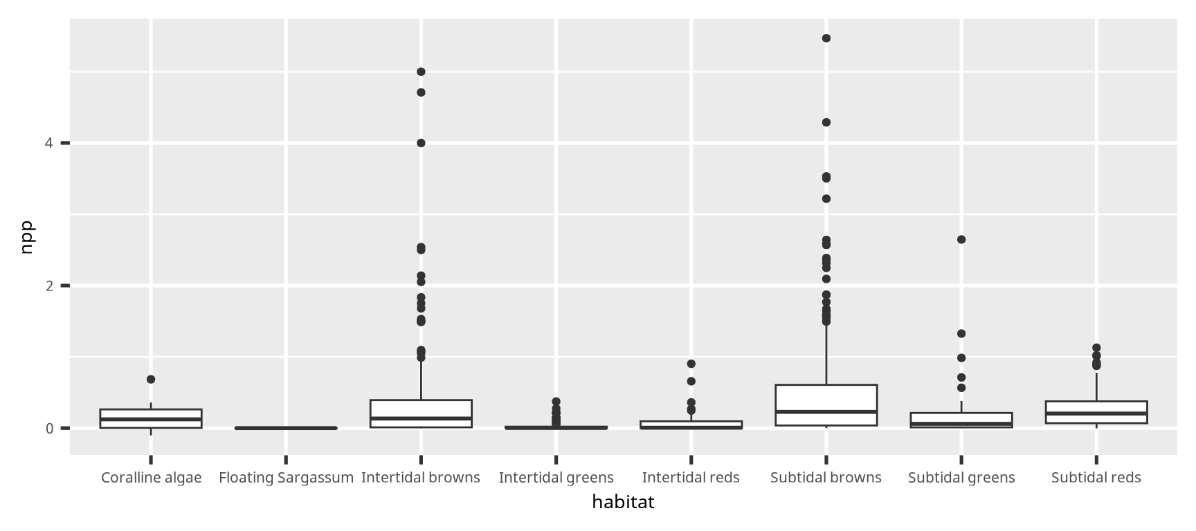
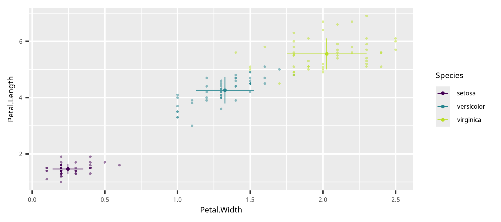
The median (中央値・メディアン) is another statistic to describe data. It is the midpoint of data that is sorted from small to large values. When the number of data is odd, the median is the value at the midpoint. When the number of data is even, the median is the average of the two values nearest to the middle.

set.seed(2020)
x = sample(1:9, size = 5, replace = TRUE)
sort(x)

[1] 1 1 6 7 8

The value in the middle is 6 so the median is 6.

median(x)

[1] 6

set.seed(2020)
x = sample(1:9, size = 4, replace = TRUE)
sort(x)

[1] 1 6 7 8

median(x)

[1] 6.5

The two values near the middle are 6 and 7, so the median is \((6 + 7) / 2 = 6.5\).

Mode (最頻値・モード)

The mode is the most common value in a dataset.

set.seed(2020)
x = sample(1:9, size = 100, replace = TRUE)
z = table(x) %>% as_tibble() %>% arrange(desc(n))
z

# A tibble: 9 × 2
  x         n
  <chr> <int>
1 8        15
2 1        14
3 2        14
4 4        13
5 6        12
6 7        10
7 3         8
8 5         8
9 9         6

The value 8 occurs 15 times, so it is the mode.

Median Absolute Deviation (中央絶対偏差)

The median absolute deviation (MAD, 中央絶対偏差) is another measure of variation.

\[ MAD = \text{median}(|x_i - \tilde{x}|) \]

\(\tilde{x}\) is the median.

mad = function(x) {
  xtilde = median(x)
  median(abs(x - xtilde))
}
x = rnorm(100)
list(mad = mad(x), sd = sd(x))

$mad
[1] 0.6588682

$sd
[1] 0.9770429

Quantile (四分位数・クォンタイル)

There are many ways to define the quantile (四分位数・クォンタイル). In any case, we first need to sort the values from smallest to largest. Then we separate the values in to four groups. The value used to separate the groups are called the quantile.

set.seed(2020)
x = sample(20:40, size = 9, replace = TRUE)
z = sort(x)
z

[1] 20 23 25 27 29 31 32 36 36

# 文科省の定義：
N = length(z)
Q1 = median(z[1:(floor(N/2))])
Q2 = median(z)
Q3 = median(z[(ceiling(N/2)+1):N])
c(min(z), Q1, Q2, Q3, max(z))

[1] 20 24 29 34 36

# R では, Tukey の定義で計算します。
quantile(z)

  0%  25%  50%  75% 100% 
  20   25   29   32   36 

In this boxplot, the whiskers indicate the minimum and maximum values. The line in the center of the box is the median (i.e., second quantile, 第2四分位数). The bottom edge of the box is the first quantile (第1四分位数) and the top edge of the box is the third quantile (第3四分位数). The distance between the first and third quantile is called the Inter-Quantile Range (IQR, 四分位範囲).

Quantile in R

set.seed(2021)
z = rpois(100, 10) 
quantile(z)

  0%  25%  50%  75% 100% 
   3    7    9   12   25 

In the standard boxplot, the dots beyond the whiskers indicate outliers. The whiskers extend to the largest value within 1.5 times the IQR from the each edge.

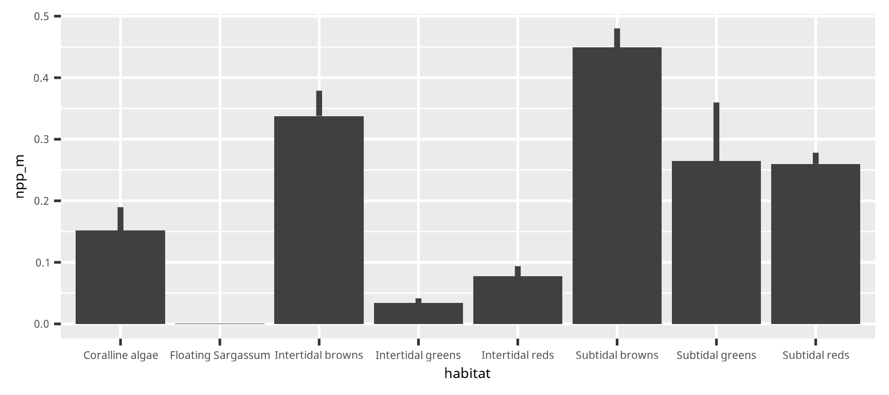
データの可視化

Data

Duarte et al. 2022. Global estimates of the extent and production of macroalgal forests. Global Ecology and Biogeography 31 (7): 1422 - 1439. https://doi.org/10.1111/geb.13515

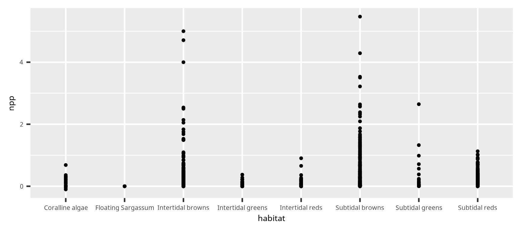
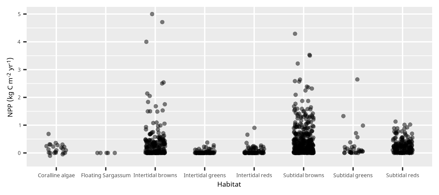
散布図 (scatter plot)

ggplot(dset) + 
  geom_point(aes(x = habitat, y = npp))

散布図 (scatter plot)

横軸は因子 (factor)、または離散変数 (discrete variable)

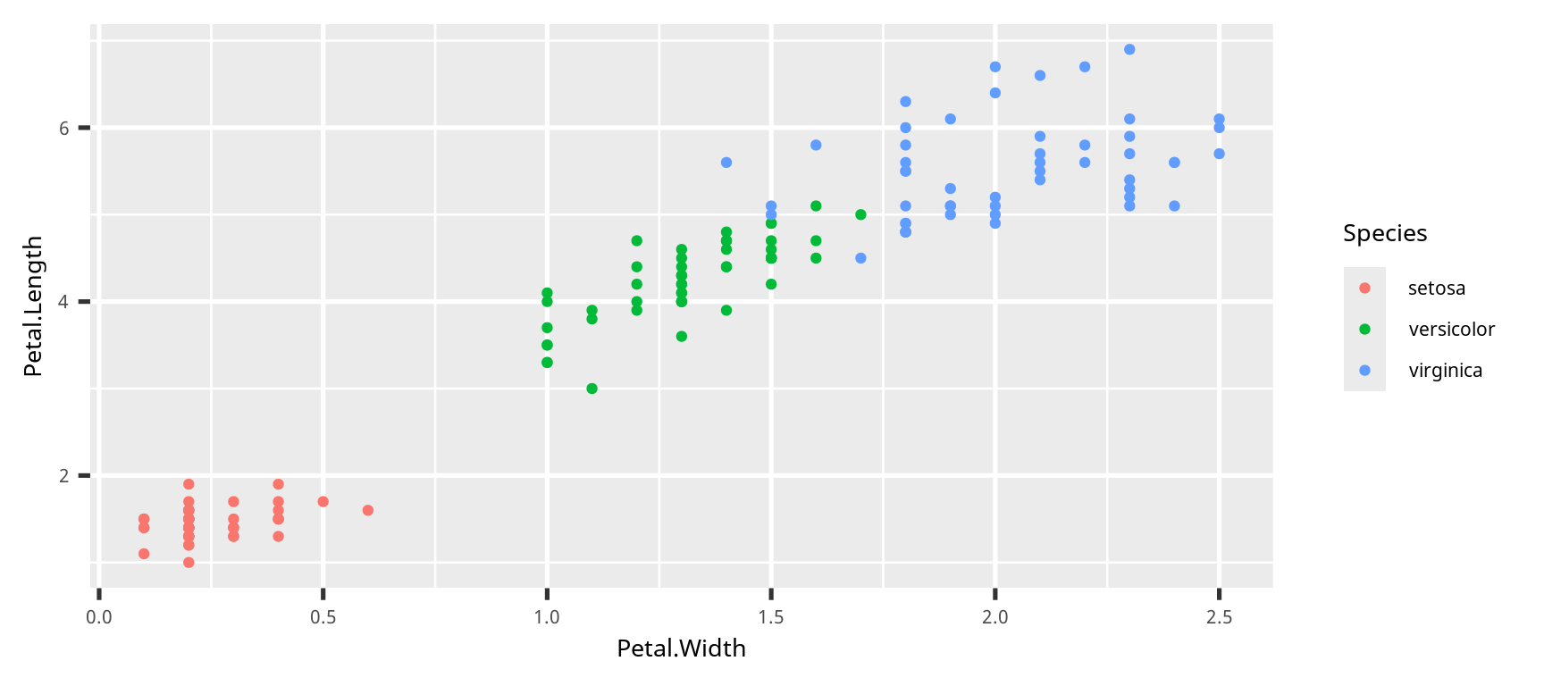
散布図とジッター (scatter plot with jitter)

ggplot(dset) + 
  geom_point(aes(x = habitat, y = npp),
             position = position_jitter(0.2))

この図の完成度は低い

散布図とジッター (scatter plot with jitter)

散布図とジッター (scatter plot with jitter)

xlabel = "Habitat"
ylabel = "NPP (kg C m<sup>-2</sup> yr<sup>-1</sup>)"
ybreaks = seq(0, 5, by = 1)
ggplot(dset) + 
  geom_point(aes(x = habitat, y = npp),
             position = position_jitter(0.2),
             alpha = 0.5,
             size = 3,
             stroke = 0) +
  scale_x_discrete(xlabel) + 
  scale_y_continuous(ylabel, 
                   breaks = ybreaks, 
                   limits = range(ybreaks) + c(-0.25, 0)) +
  theme(axis.title.y = element_markdown())

散布図とジッター (scatter plot with jitter)

箱ひげ図 (box plot)

ggplot(dset) + 
  geom_boxplot(aes(x = habitat, y = npp))

箱ひげ図 (box plot)

点とエラーバー (point and error bar)

# Calculate the mean, standard deviation (sd),
# then number of samples (length), and the standard error.

dset2 = 
  dset |> 
  group_by(habitat) |> 
  summarise(across(npp, 
                   list(m = mean, sd = sd, n = length))) |> 
  mutate(npp_se = npp_sd / sqrt(npp_n - 1))

ggplot(dset2) + 
  geom_point(aes(x = habitat, y = npp_m)) +
  geom_errorbar(aes(x = habitat, 
                    ymin = npp_m - npp_sd,
                    ymax = npp_m + npp_sd),
                width = 0.25)

点とエラーバー (point and error bar)

エラーバーは１標準偏差

点とエラーバー (point and error bar)

# Calculate the mean, standard deviation (sd),
# then number of samples (length), and the standard error.

dset2 = 
  dset |> 
  group_by(habitat) |> 
  summarise(across(npp, 
                   list(m = mean, sd = sd, n = length))) |> 
  mutate(npp_se = npp_sd / sqrt(npp_n - 1))

ggplot(dset2) + 
  geom_point(aes(x = habitat, y = npp_m)) +
  geom_errorbar(aes(x = habitat, 
                    ymin = npp_m - npp_se,
                    ymax = npp_m + npp_se),
                width = 0.25)

点とエラーバー (point and error bar)

エラーバーは１標準誤差

棒グラフ (bar graph)

dset2 = 
  dset |> 
  group_by(habitat) |> 
  summarise(across(npp, 
                   list(m = mean, sd = sd, n = length))) |> 
  mutate(npp_se = npp_sd / sqrt(npp_n - 1))

ggplot(dset2) + 
  geom_col(aes(x = habitat, y = npp_m))

棒グラフ (bar graph)

棒グラフとエラーバー (candle stick graph)

dset2 = 
  dset |> 
  group_by(habitat) |> 
  summarise(across(npp, 
                   list(m = mean, sd = sd, n = length))) |> 
  mutate(npp_se = npp_sd / sqrt(npp_n - 1))

ggplot(dset2) + 
  geom_col(aes(x = habitat, y = npp_m),
           fill = "grey25") + 
  geom_errorbar(aes(x = habitat,
                    ymin = npp_m,
                    ymax = npp_m + npp_sd), 
                width = 0,
                linewidth = 2, 
                color = "grey25")

棒グラフとエラーバー (candle stick graph)

エラーバーは１標準偏差

棒グラフとエラーバー (candle stick graph)

dset2 = 
  dset |> 
  group_by(habitat) |> 
  summarise(across(npp, 
                   list(m = mean, sd = sd, n = length))) |> 
  mutate(npp_se = npp_sd / sqrt(npp_n - 1))

ggplot(dset2) + 
  geom_col(aes(x = habitat, y = npp_m),
           fill = "grey25") + 
  geom_errorbar(aes(x = habitat,
                    ymin = npp_m,
                    ymax = npp_m + npp_se), 
                width = 0,
                linewidth = 2, 
                color = "grey25")

棒グラフとエラーバー (candle stick graph)

エラーバーは１標準誤差

棒グラフとエラーバー (candle stick graph)

dset2 = 
  dset |> 
  group_by(habitat) |> 
  summarise(across(npp, 
                   list(m = mean, sd = sd, n = length))) |> 
  mutate(npp_se = npp_sd / sqrt(npp_n - 1)) |> 
  mutate(habitat = fct_reorder(habitat, npp_m, .desc = TRUE))

ggplot(dset2) + 
  geom_col(aes(x = habitat, y = npp_m),
           fill = "grey25") + 
  geom_errorbar(aes(x = habitat,
                    ymin = npp_m,
                    ymax = npp_m + npp_se), 
                width = 0,
                linewidth = 2, 
                color = "grey25")

棒グラフとエラーバー (candle stick graph)

エラーバーは１標準偏差、データを降順に並べ替えた

散布図 (scatter plot)

ggplot(iris) + 
  geom_point(aes(x = Petal.Width, y = Petal.Length))

散布図 (scatter plot)

横軸も連続変数(continuous variable)

散布図 (scatter plot)

ggplot(iris) + 
  geom_point(aes(x = Petal.Width, y = Petal.Length, 
                 color = Species))

散布図 (scatter plot)

横軸も連続変数(continuous variable)

折れ線グラフ (line graph)

se = function(x) {sd(x) / sqrt(length(x) -1)}
iris |> 
  group_by(Species,
           Petal.Width) |> 
  summarise(across(Petal.Length,
                   list(m = mean, sd = sd, se = se))) |> 
  ggplot() + 
  geom_point(aes(x = Petal.Width, 
                 y = Petal.Length_m, 
                 color = Species)) +
  geom_line(aes(x = Petal.Width,
                y = Petal.Length_m, 
                color = Species))

折れ線グラフ (line graph)

横軸も連続変数(continuous variable)

折れ線グラフ (line graph)

se = function(x) {sd(x) / sqrt(length(x) -1)}
iris |> 
  group_by(Species,
           Petal.Width) |> 
  summarise(across(Petal.Length,
                   list(m = mean, sd = sd, se = se))) |> 
  ggplot() + 
  geom_line(aes(x = Petal.Width,
                y = Petal.Length_m, 
                color = Species)) +
  geom_errorbar(aes(x = Petal.Width,
                    ymin = Petal.Length_m - Petal.Length_se,
                    ymax = Petal.Length_m + Petal.Length_se,
                    color = Species),
                linewidth = 2,
                width = 0.0) +
  geom_errorbar(aes(x = Petal.Width,
                    ymin = Petal.Length_m - Petal.Length_sd,
                    ymax = Petal.Length_m + Petal.Length_sd,
                    color = Species),
                width = 0.0)

折れ線グラフ (line graph)

１標準偏差（細線）と１標準誤差（太線）を示した

点とエラーバー (point and error bar)

iris |> 
  group_by(Species) |> 
  summarise(across(matches("Petal"),
                   list(m = mean, sd = sd, n = length))) |> 
  mutate(Petal.Width_se = Petal.Width_sd / sqrt(Petal.Width_n - 1)) |> 
  mutate(Petal.Length_se = Petal.Length_sd / sqrt(Petal.Length_n - 1)) |> 
  ggplot() + 
  geom_point(aes(x = Petal.Width_m, 
                 y = Petal.Length_m, 
                 color = Species)) +
  geom_errorbarh(aes(y = Petal.Length_m,
                     xmin = Petal.Width_m - Petal.Width_sd,
                     xmax = Petal.Width_m + Petal.Width_sd,
                     color = Species),
                 height = 0.0)+
  geom_errorbar(aes(x = Petal.Width_m,
                    ymin = Petal.Length_m - Petal.Length_sd,
                    ymax = Petal.Length_m + Petal.Length_sd,
                    color = Species),
                width = 0.0)

点とエラーバー (point and error bar)

横軸も連続変数(continuous variable)

点とエラーバー (point and error bar)

iris |> 
  group_by(Species) |> 
  summarise(across(matches("Petal"),
                   list(m = mean, sd = sd, n = length))) |> 
  mutate(Petal.Width_se = Petal.Width_sd / sqrt(Petal.Width_n - 1)) |> 
  mutate(Petal.Length_se = Petal.Length_sd / sqrt(Petal.Length_n - 1)) |> 
  ggplot() + 
  geom_point(aes(x = Petal.Width,
                 y = Petal.Length,
                 color = Species),
             data = iris,
             stroke = 0,
             alpha = 0.5) +
  geom_point(aes(x = Petal.Width_m, 
                 y = Petal.Length_m, 
                 color = Species)) +
  geom_errorbarh(aes(y = Petal.Length_m,
                     xmin = Petal.Width_m - Petal.Width_sd,
                     xmax = Petal.Width_m + Petal.Width_sd,
                     color = Species),
                 height = 0.0)+
  geom_errorbar(aes(x = Petal.Width_m,
                    ymin = Petal.Length_m - Petal.Length_sd,
                    ymax = Petal.Length_m + Petal.Length_sd,
                    color = Species),
                width = 0.0) +
  scale_color_viridis_d(end = 0.9)

点とエラーバー (point and error bar)

変数ごとの平均値と１標準偏差も示した