Principal Component Analysis

Greg Nishihara

2024 / 07 / 07

Redundancy Analysis

Principal component analysis (PCA) is a method to find new variables (i.e., principal components) that are linear functions of the original variables. The new variable should successively maximizes variance and should not be correlated with each other. The principal components are found by eigenanalysis (Jolliffe and Cadima 2016; Hotelling 1933; Pearson 1901).

Principal component analysis (PCA)

PCA¹ is the eigenanalysis² of the \(p\times p\) variance – covariance matrix³ \(\Sigma\)

\[ \mathbf{\Sigma} = \frac{\mathbf{Y_c}^\top \mathbf{Y_c}}{n-1} \]

\(\mathbf{Y}_c\) is the column-centered matrix of the orignal data \(\mathbf{Y}\). \(n\) is the number of rows in \(\mathbf{Y}_c\).

1. 主成分分析

2. 固有値解析

3. 分散共分散行列

Definition of \(\mathbf{Y_c}\)

\[ \overbrace{\begin{bmatrix}2.25 & 2.00 & 2.00\\-1.75 & 0.00 & -2.00\\ 0.25 & -1.00 & -2.00\\-0.75 & -1.00 & 2.00\end{bmatrix}}^{\mathbf{Y_c}} = \overbrace{\begin{bmatrix}5 & 4 & 5\\1 & 2 & 1\\3 & 1 & 1\\2 & 1 & 5\end{bmatrix}}^{\mathbf{Y}} - \overbrace{\begin{bmatrix}2.75 & 2.00 & 3.00\\2.75 & 2.00 & 3.00\\2.75 & 2.00 & 3.00\\2.75 & 2.00 & 3.00\end{bmatrix}}^{\overline{\mathbf{Y}}} \]

\(\mathbf{Y}\) is the original data, \(\overline{\mathbf{Y}}\) is the column-means of \(\mathbf{Y}\).

Decomposition of \(\mathbf{Y_c}\)

The eigenanalysis of \(\Sigma\) is defined as the following:

\[ \frac{\mathbf{Y_c}^\top \mathbf{Y_c}}{n-1} = \mathbf{\Sigma} = \mathbf{V}_{pca}\mathbf{L}\mathbf{V}_{pca}^\top \]

where, \(\mathbf{V}_{pca} = \begin{bmatrix}\mathbf{v_1} & \mathbf{v_2} & \cdots & \mathbf{v_p}\end{bmatrix}\) is a matrix of \(p\) eigenvectors¹ and \(\mathbf{L}\) is a diagonal matrix of the eigenvalues². Each \(\mathbf{v_i}\) is also known as the \(i\)th principal component³.

1. 固有ベクトル

2. 固有値

3. 主成分

Eigenvalue

The eigenvalue matrix is a \(p\times p\) diagonal matrix¹.

\[ \mathbf{L} = \begin{bmatrix} \lambda_1 & 0 & 0 & \cdots & 0 \\ 0 & \lambda_2 & 0 & \cdots & 0 \\ \vdots & & \ddots & \ & \vdots \\ 0 & 0 & 0 & \cdots & \lambda_p \\ \end{bmatrix} \]

Recall that \(p\) is the number of variables (i.e., columns) in \(\mathbf{Y_c}\)

1. 対角行列

Singular value decomposition

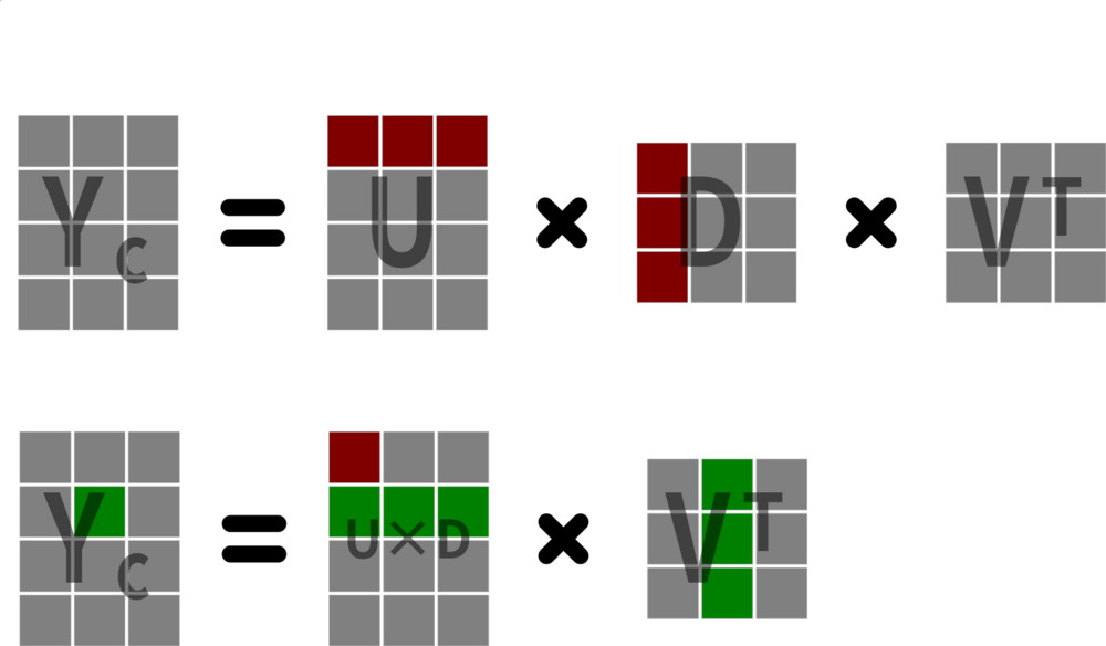
Instead of solving \(\frac{\mathbf{Y_c}^\top \mathbf{Y_c}}{n-1} = \mathbf{\Sigma} = \mathbf{V}_{pca}\mathbf{L}\mathbf{V}_{pca}^\top\) (i.e., eigenanalysis¹), it is easier to do a singular value decomposition (SVD)².

\[ \mathbf{Y_c} = \mathbf{U}\mathbf{D}\mathbf{V}_{svd}^\top \]

1. 固有値解析

2. 特異値分解

SVD

\[ \mathbf{Y_c} = \mathbf{U}\mathbf{D}\mathbf{V}_{svd}^\top \]

\(\mathbf{U}\) is the left singular vectors¹ of \(\mathbf{Y_c}\) and are the eigenvectors of \(\mathbf{Y_c}\mathbf{Y_c}^\top\).

1. 左特異値ベクトル

SVD

\[ \mathbf{Y_c} = \mathbf{U}\mathbf{D}\mathbf{V}_{svd}^\top \]

\(\mathbf{D}\) is a diagonal matrix of the singular values¹.

1. 特異値

SVD

\[ \mathbf{Y_c} = \mathbf{U}\mathbf{D}\mathbf{V}_{svd}^\top \]

\(\mathbf{V}_{svd}\) is the right singular vectors¹ of \(\mathbf{Y_c}\) and are the eigenvectors of \(\mathbf{Y_c}^\top\mathbf{Y_c}\).

Note that \(\mathbf{V}_{pca} \approx \mathbf{V}_{sda}\).

1. 右特異値ベクトル

Solving for \(\mathbf{L}\)

To find the eigenvalue, we must solve for \(\mathbf{\Sigma}\).

\[ \mathbf{\Sigma} = \frac{\mathbf{Y_c}^\top \mathbf{Y_c}}{n-1 } \]

\[ \mathbf{Y_c} = \mathbf{U}\mathbf{D}\mathbf{V}_{svd}^\top \]

Substitute \(\mathbf{Y_c}\) in to \(\mathbf{\Sigma}\)

\[ \begin{aligned} \mathbf{\Sigma} &= \frac{\mathbf{Y_c}^\top \mathbf{Y_c}}{n-1 }\\ & \mathbf{Y_c} = \mathbf{U}\mathbf{D}\mathbf{V}_{svd}^\top \\ \mathbf{\Sigma} &= \frac{(\mathbf{U}\mathbf{D}\mathbf{V}_{svd}^\top )^\top (\mathbf{D}\mathbf{S}\mathbf{V}_{svd}^\top )}{n-1 } \\ \mathbf{\Sigma} &= \frac{\mathbf{V}_{svd}\mathbf{D}^\top\mathbf{U}^\top \mathbf{U} \mathbf{D} \mathbf{V}_{svd}^\top}{n-1 }\\ \end{aligned} \]

Substitute \(\mathbf{Y_c}\) in to \(\mathbf{\Sigma}\)

Since \(\mathbf{U}^\top\mathbf{U}=1\),

\[ \mathbf{\Sigma} = \frac{\mathbf{V}_{svd}\mathbf{D}^\top \mathbf{D} \mathbf{V}_{svd}^\top}{n-1 } = \mathbf{V}_{pca}\mathbf{L}\mathbf{V}_{pca}^\top \]

and \(\mathbf{V}^\top\mathbf{V}=1\),

\[ \mathbf{\Sigma} = \frac{\mathbf{D}^\top\mathbf{D}}{n-1} = \mathbf{L} \]

or more simply, \(\lambda_i = \frac{d_i^2}{n-1}\).

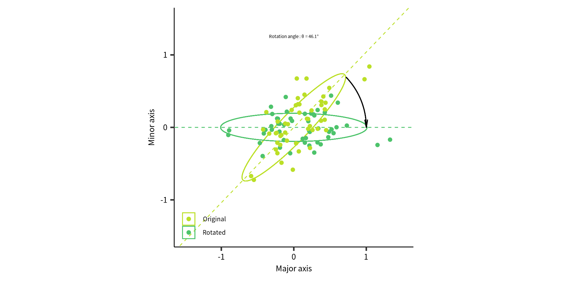
Visualize what we want to do

The rotation angle \(\theta\) can also be determined from the rotation vector as follows: \(\mathbf{V}_\text{svd} = \begin{bmatrix} \cos\theta & -\sin\theta\\ \sin\theta & \cos\theta\\ \end{bmatrix}\).

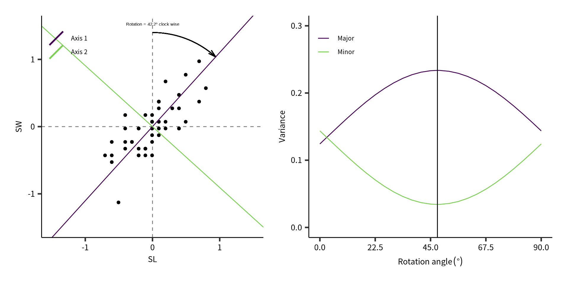
Computation mechanics

Apply SVD to the previous example results in the following equation.

\[ \overbrace{\begin{bmatrix}2.25 & 2.00 & 2.00\\-1.75 & 0.00 & -2.00\\ 0.25 & -1.00 & -2.00\\-0.75 & -1.00 & 2.00\end{bmatrix}}^{\mathbf{Y_c}} = \overbrace{\begin{bmatrix}-0.73 & 0.43 & -0.15\\ 0.526 & 0.078 & -0.683\\0.39 & 0.33 & 0.70\\-0.18 & -0.84 & 0.13\end{bmatrix} }^{\mathbf{U}}\times \overbrace{\begin{bmatrix}4.66 & 0.00 & 0.00\\0.00 & 2.63 & 0.00\\0.00 & 0.00 & 1.47\end{bmatrix} }^{\mathbf{D}}\times \overbrace{\begin{bmatrix}-0.50 & -0.36 & -0.79\\ 0.59 & 0.52 & -0.62\\ 0.633 & -0.772 & -0.051\end{bmatrix} }^{\mathbf{V}^\top} \]

Example 1: determine \(\mathbf{Y_c}\)

Calculate the centered data matrix.

Y = iris[1:50, 1:2]
colnames(Y) = colnames(iris)[1:2] |> 
  str_remove_all("[a-z|\\.]+") 
nm = dim(Y)
Ybar = apply(Y, 2, mean)
Ybar = matrix(Ybar, ncol = nm[2], 
              nrow = nm[1],
              byrow = TRUE)
Yc = Y - Ybar
Yc |> head()

      SL     SW
1  0.094  0.072
2 -0.106 -0.428
3 -0.306 -0.228
4 -0.406 -0.328
5 -0.006  0.172
6  0.394  0.472

Example 1: SVD

Calculate the eigenvectors, eigenvalues, and singular values using svd().

svdout = svd(Yc)
umat = svdout$u  # Left singular vectors
vmat = svdout$v  # Right singular vectors (i.e., eigenvectors)
d = svdout$d     # Singular values
n = nm[1]        # Data rows
p = nm[2]        # Data columns (i.e., variables)

Example 1: eigenvalues

Recall that,

\[ \lambda_i = \frac{d_i^2} {n-1} \]

# lambda = ((diag(d) %*% t(diag(d))) / (n - 1)) |> diag()
lambda = d^2 / (n - 1)

Therefore, the eigenvalues are 0.2337 and 0.0343.

Example 1: eigenvectors

rownames(vmat) = colnames(Yc)
colnames(vmat) = str_glue("PC{1:p}")

The eigenvectors are:

vmat

          PC1        PC2
SL -0.6717496 -0.7407783
SW -0.7407783  0.6717496

Example 1: mechanics of rotating \(\mathbf{Y_c}\)

The eigenvectors indicate the direction of the vectors that maximizes the variance of each axis. In this case, maximizing the variance in one axis lead to a minimization in the other.

Example 1: derived information

The total variance before rotation is:

diag(var(Yc)) |> sum()

[1] 0.2679388

and should be the same as the total inertia (i.e., variance) after rotation:

sum(lambda)

[1] 0.2679388

The variance of SL and SW is:

diag(var(Yc))

       SL        SW 
0.1242490 0.1436898 

Example 1: more derived information

The relative importance of SL and SW is:

diag(var(Yc)) / sum(diag(var(Yc)))

       SL        SW 
0.4637215 0.5362785 

However, the variance of the principal components and their relative importance is different:

lambda # The variance

[1] 0.23366074 0.03427804

importance = lambda / sum(lambda)
names(importance) = colnames(vmat)
importance # The relative importance

      PC1       PC2 
0.8720677 0.1279323 

The relative importance indicates the proportion of variation explained by the principal component axis. Conceptually, \(\mathbf{Y_c}\) is rotated until each component is maximized successively.

Example 1: scores and loadings

Scores¹ are the data points projected onto the principal component axes.

# There are a total of n = 50 scores.
scores = umat %*% diag(d)
colnames(scores) = str_c("PC", 1:ncol(scores))
scores |> head()

            PC1         PC2
[1,] -0.1164805 -0.02126719
[2,]  0.3882586 -0.20898631
[3,]  0.3744528  0.07351926
[4,]  0.5157056  0.08042214
[5,] -0.1233834  0.11998560
[6,] -0.6143167  0.02519914

1. 主成分得点: あるデータ点を主成分ベクトルで表現した場合の値

Example 1: scores and loadings

Loadings (rescaled loadings)¹ indicates the relationship of the variable with the principal component axes.

loadings = (vmat %*% diag(d)) / sqrt(n-1)
colnames(loadings) = str_glue("PC{1:p}")
loadings

          PC1        PC2
SL -0.3247134 -0.1371501
SW -0.3580809  0.1243699

Therefore, for variable SL, the loadings on PC1 and PC2 are -0.325 and -0.137, respectively. The cosine of the angle between loadings are their correlation.

SL = loadings[1, ]
SW = loadings[2, ]
L1 = atan2(y = SL[2], x = SL[1])
L2 = atan2(y = SW[2], x = SW[1])
theta = abs(L1 - L2)
cos(theta)

      PC2 
0.7425467 

1. 主成分負荷量: ある主成分ベクトルのデータ点に対する重み

Example 2: vegan::rda()

First run the analysis with both rda() and `svd().

rdaout = rda(Yc)
svdout = svd(Yc)

Left singular matrix¹

svdout$u |> head(n = 2)     # SDV result
rdaout$CA$u |> head(n = 2)  # RDA result

            [,1]        [,2]
[1,] -0.03442408 -0.01640983
[2,]  0.11474404 -0.16125450
          PC1         PC2
1 -0.03442408 -0.01640983
2  0.11474404 -0.16125450

Right singular matrix²

svdout$v |> head(n = 2)    # SDV result
rdaout$CA$v |> head(n = 2) # RDA result

           [,1]       [,2]
[1,] -0.6717496 -0.7407783
[2,] -0.7407783  0.6717496
          PC1        PC2
SL -0.6717496 -0.7407783
SW -0.7407783  0.6717496

1. 左特異値ベクトル

2. 右特異値ベクトル

Example 2: vegan::rda()

Eigenvalues

(svdout$d^2)/(n-1) # SDV result
rdaout$CA$eig      # RDA result

[1] 0.23366074 0.03427804
       PC1        PC2 
0.23366074 0.03427804 

Example 2: similar output

rdaout |> summary(display = NA)

Call:
rda(X = Yc) 

Partitioning of variance:
              Inertia Proportion
Total          0.2679          1
Unconstrained  0.2679          1

Eigenvalues, and their contribution to the variance 

Importance of components:
                         PC1     PC2
Eigenvalue            0.2337 0.03428
Proportion Explained  0.8721 0.12793
Cumulative Proportion 0.8721 1.00000

Scaling 2 for species and site scores
* Species are scaled proportional to eigenvalues
* Sites are unscaled: weighted dispersion equal on all dimensions
* General scaling constant of scores:  

• Note the total inertia is the sum of the eigenvalues 0.268.
• The proportion explained is the ratio of the eigenvalues to the sum of the eigenvalues \((\lambda_i / \sum{\lambda_i})\).

At this stage numeric results from svd() and rda() are equivalent. However, the scores and loadings are scaled differently.

Example 2: vegan-like analysis

In vegan::rda(), the scores are scaled according to the following:

• scaling = 1:¹ \(C\sqrt{\lambda_i / \sum\lambda_i}\)
• scaling = 2:² \(C\)

The constant term is \(C = \sqrt[4]{(n -1)\sum{\lambda_i}}\).

See the decision-vegan.pdf vignette for details.

const = ((n - 1) * sum(lambda))^{1/4}
scale1 = sqrt(lambda / sum(lambda) ) * const
scale2 = const
umat1 = umat %*% diag(scale1)
umat2 = umat * scale2
vmat1 = vmat %*% diag(scale1)
vmat2 = vmat * scale2

1. Interpret spatial patterns.

2. Interpret vector directions and angles.

Example 2: scaling = 1 and 2

Scaling 1

\[ \mathbf{U}_1 = \mathbf{U} \times \begin{bmatrix} \frac{\sqrt{\lambda_1}}{\sum\lambda_k} & 0 & 0 & \cdots & 0\\ 0 & \frac{\sqrt{\lambda_2}}{\sum\lambda_k} & 0 & \cdots & 0\\ 0 & 0 & \ddots & \cdots & 0 \\ 0 & 0 & 0 & \cdots & \frac{\sqrt{\lambda_k}}{\sum\lambda_k} \\ \end{bmatrix} \times \sqrt[4]{(n -1)\sum{\lambda_k}} \]

Scaling 2

\[ \mathbf{U}_2 = \mathbf{U} \times \sqrt[4]{(n -1)\sum{\lambda_k}} \]

\(\mathbf{U}_1\) and \(\mathbf{U}_2\) are the scaled scores.

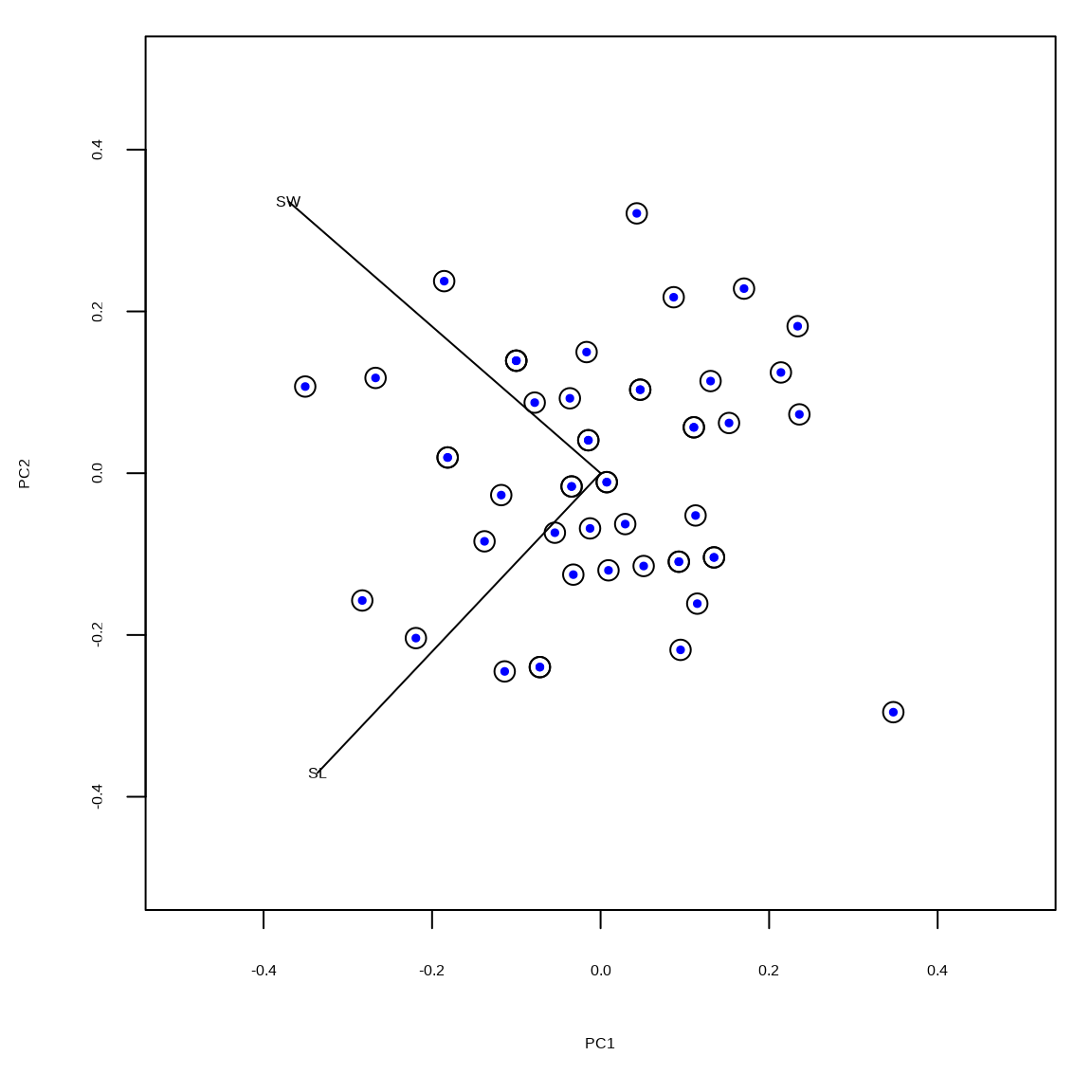
Example 2: no scaling

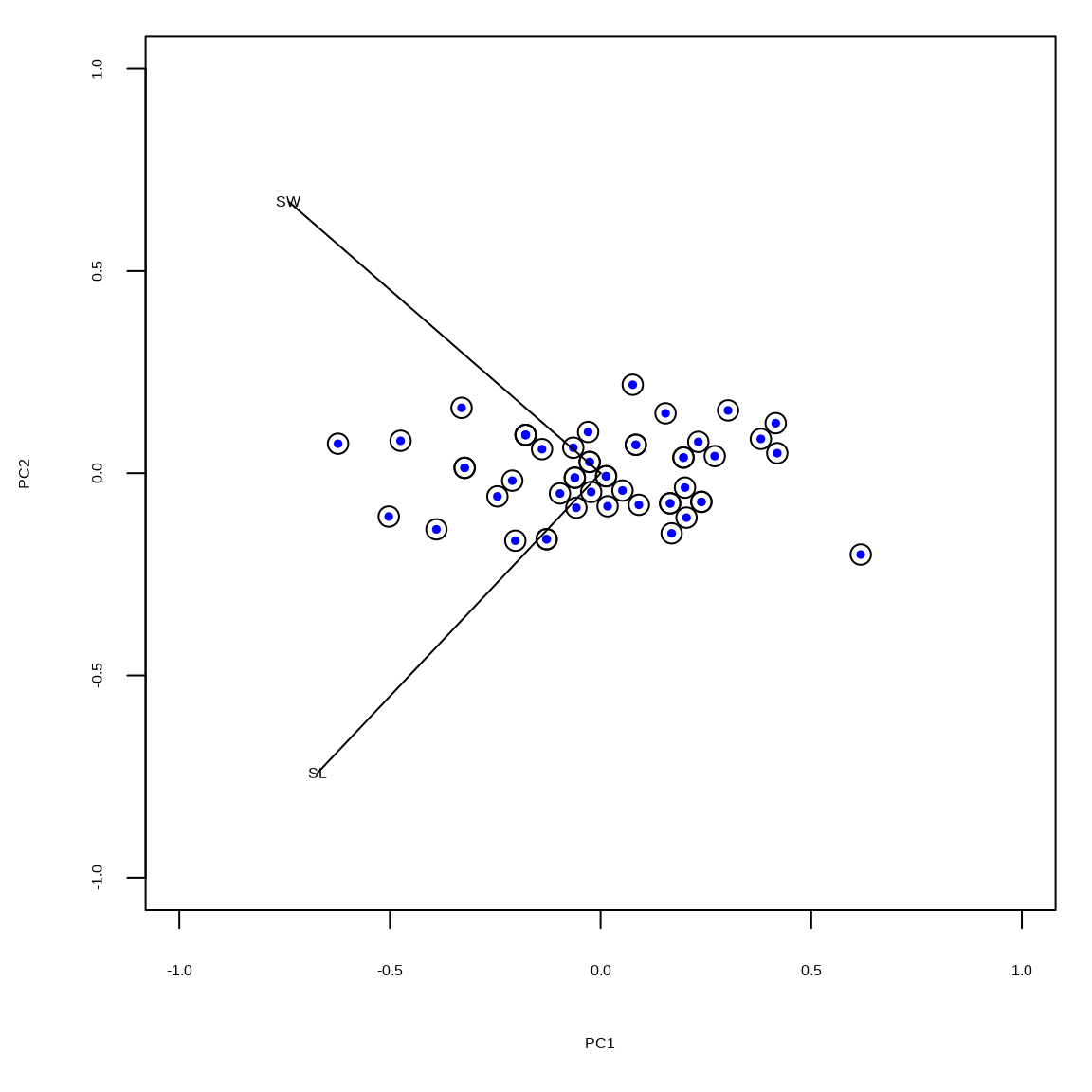
The unscaled principal components are in the matrix \(\mathbf{U}\). The black circles indicate the vegan::rda() output and the colored dots indicate the results based on the SVD.

limits = c(-0.5, 0.5)
tmp = scores(rdaout, scaling = "none", display = "species")
tmp = tmp %*% diag(1/diag(sqrt(tmp %*% t(tmp)))) / 2
scores(rdaout, scaling = "none", display = "sites") |> 
  plot(cex = 1.5, xlim = limits, ylim = limits)
points(umat[,1], umat[,2], pch = 19, col = "blue", cex = 0.5)
segments(c(0,0), c(0,0), tmp[,1], tmp[,2])
text(tmp[,1], tmp[,2], labels = rownames(tmp))

Example 2: scaling 1

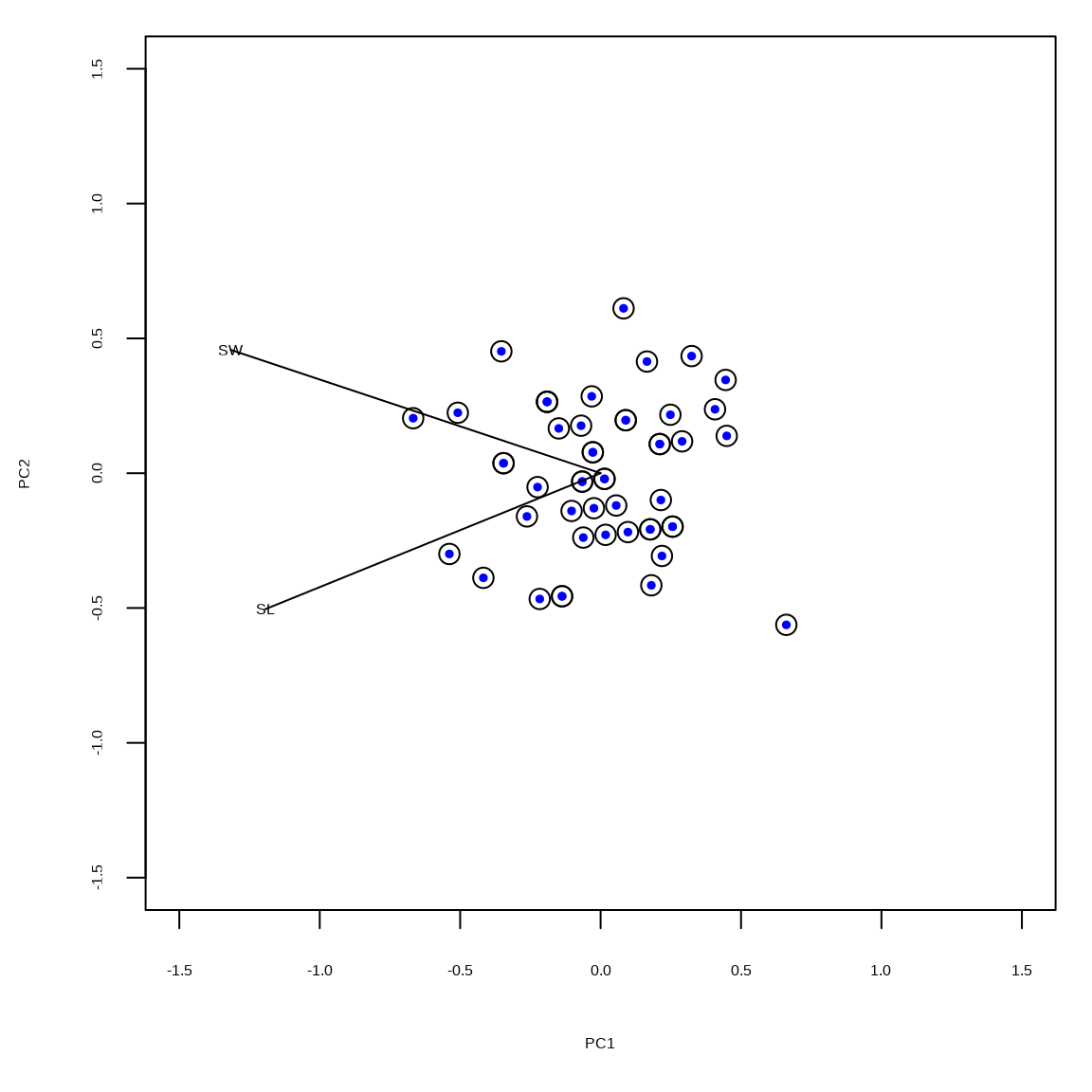
The scaled principal components are in the matrix \(\mathbf{U}_1\). The black circles indicate the vegan::rda() output and the colored dots indicate the results based on the SVD. Distances between dots indicate approximate euclidean distances \((d = \sqrt{x^2+y^2})\)¹.

limits = c(-1, 1)
tmp = scores(rdaout, scaling = 1, display = "species")
tmp = tmp %*% diag(1/diag(sqrt(tmp %*% t(tmp))))
scores(rdaout, scaling = 1, display = "sites") |> 
  plot(cex = 1.5, xlim = limits, ylim = limits)
points(umat1[,1], umat1[,2], pch = 19, col = "blue", cex = 0.5)
segments(c(0,0), c(0,0), tmp[,1], tmp[,2])
text(tmp[,1], tmp[,2], labels = rownames(tmp))

1. ユークリッド距離

Example 2: scaling 2

The scaled principal components are in the matrix \(\mathbf{U}_2\). The black circles indicate the vegan::rda() output and the colored dots indicate the results based on the SVD. Angles between vectors (radians) indicate correlation.

limits = c(-1.5, 1.5)
tmp = scores(rdaout, choices = c(1,2), scaling = 2, display = "species")
tmp = tmp %*% diag(1/diag(sqrt(tmp %*% t(tmp)))) 
scores(rdaout, scaling = 2, display = "sites") |> 
  plot(cex = 1.5, xlim = limits, ylim = limits)
points(umat2[,1], umat2[,2], pch = 19, col = "blue", cex = 0.5)
segments(c(0,0), c(0,0), tmp[,1], tmp[,2])
text(tmp[,1], tmp[,2], labels = rownames(tmp))

Example 3: unscaled 3D plot

Example 3: scaled 3D plot

Scaling = 1

Scaling = 2

Example 3: summary output

rdaout |> summary(display = NA)

Call:
rda(X = Yc) 

Partitioning of variance:
              Inertia Proportion
Total           3.992          1
Unconstrained   3.992          1

Eigenvalues, and their contribution to the variance 

Importance of components:
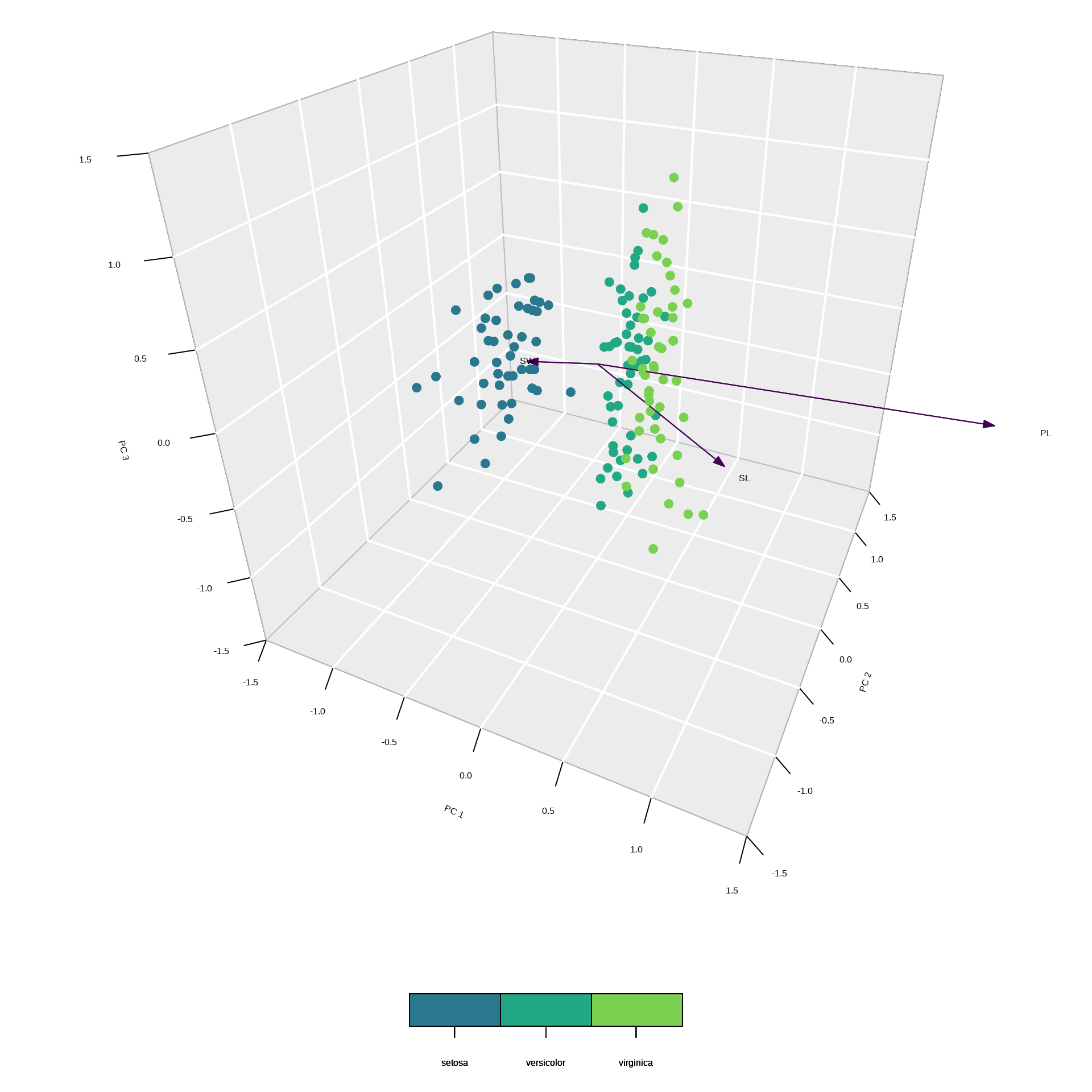
                         PC1     PC2     PC3
Eigenvalue            3.6911 0.24138 0.05945
Proportion Explained  0.9246 0.06047 0.01489
Cumulative Proportion 0.9246 0.98511 1.00000

Scaling 2 for species and site scores
* Species are scaled proportional to eigenvalues
* Sites are unscaled: weighted dispersion equal on all dimensions
* General scaling constant of scores:  

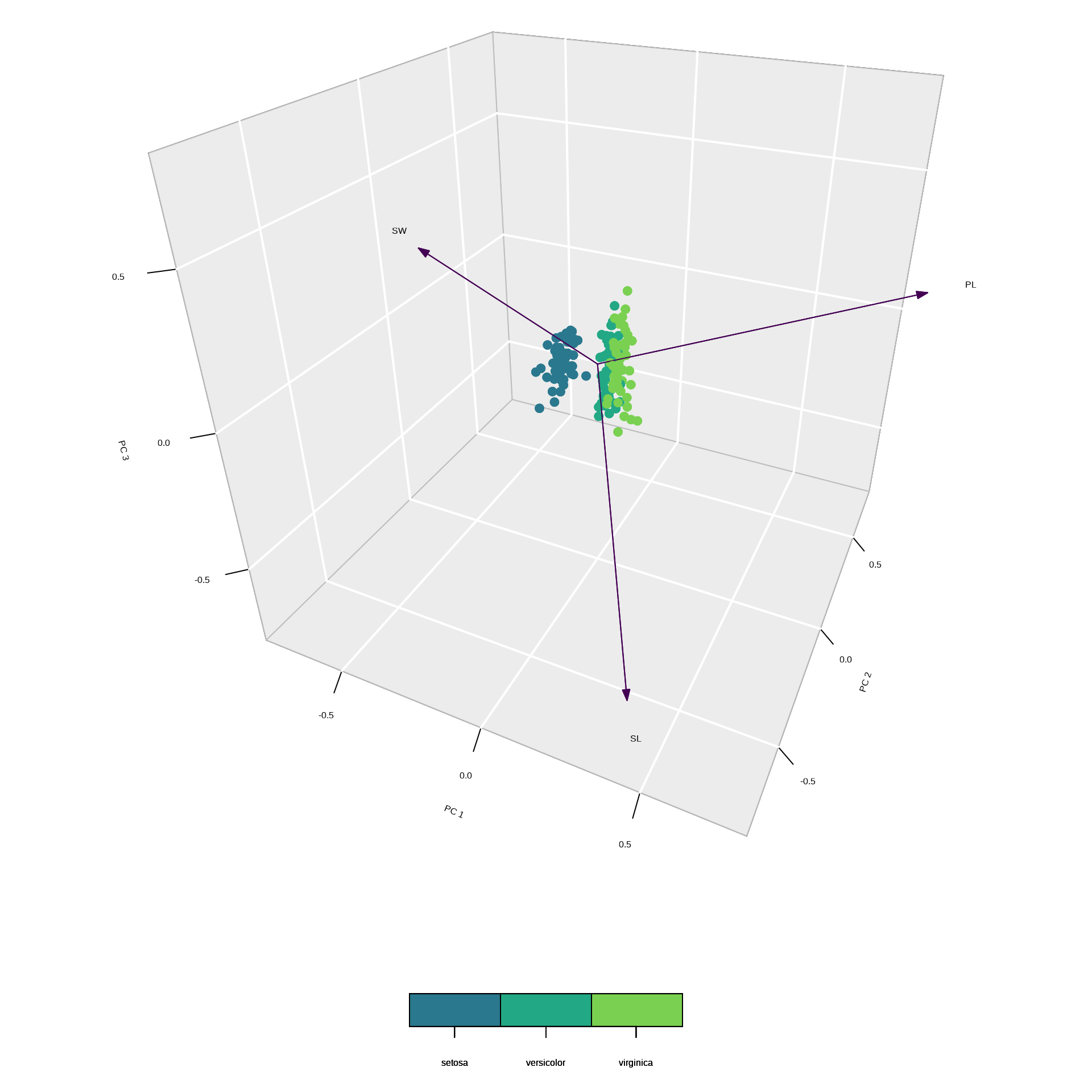
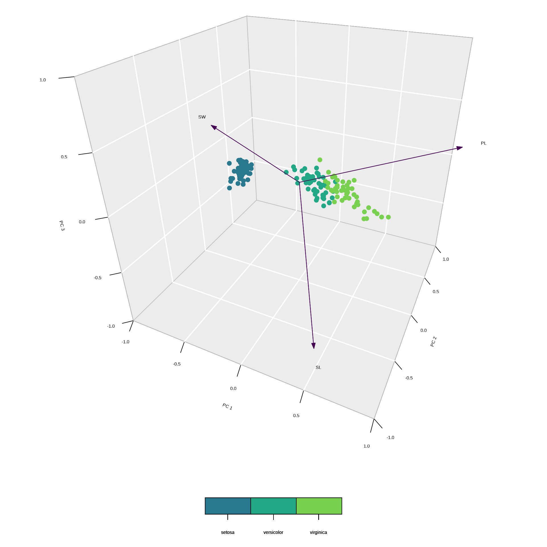
PC1 explains 92.46 % of the inertia, therefore most of the variation occurs along the PC1 axis.

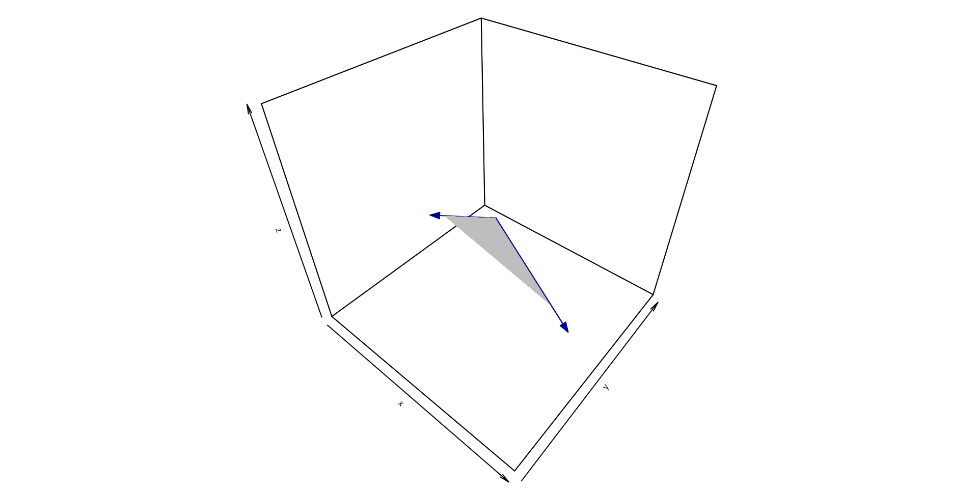
Example 4: correlations among vectors

The correlation between two vectors is determined as

\[ \begin{aligned} \cos\theta &= \frac{v_1\cdot v_2}{\lVert v_1 \rVert \lVert v_2 \rVert} \\ \sin\theta &= \frac{\lVert v_1\times v_2 \rVert}{\lVert v_1 \rVert \lVert v_2 \rVert} \\ \tan\theta &= \frac{\lVert v_1\times v_2\rVert}{v_1 \cdot v_2 } \\ \end{aligned} \]

Example 3: problem

The correlation between two vectors is the cosine of the angle between the vectors.

\[ \cos\theta = \frac{v_1\cdot v_2}{\lVert v_1 \rVert \lVert v_2 \rVert} \]

Determine the angle of the shaded region.

Example 3: partial solution

\[ \cos\theta = \frac{v_1\cdot v_2}{\lVert v_1 \rVert \lVert v_2 \rVert} \]

\[ \begin{aligned} v_1 &= \begin{bmatrix} 1.85 & -0.78 & -0.40 \end{bmatrix} \\ v_2 &= \begin{bmatrix} -0.43 & -0.90 & 0.40 \end{bmatrix} \\ \lVert v_1\rVert &= \sqrt{\begin{bmatrix} 1.85 & -0.78 & -0.40 \end{bmatrix} \begin{bmatrix} 1.85 \\ -0.78 \\ -0.40 \end{bmatrix}} = 2.05 \\ \lVert v_2\rVert &= \sqrt{\begin{bmatrix} -0.43 & -0.90 & 0.40 \end{bmatrix} \begin{bmatrix} -0.43 \\ -0.90 \\ 0.40 \end{bmatrix}} = 1.08 \\ \end{aligned} \]

Example 3: final solution

\[ \cos\theta = \frac{\begin{bmatrix} 1.85 & -0.78 & -0.40 \end{bmatrix} \begin{bmatrix} -0.43 \\ -0.90 \\ 0.40 \end{bmatrix}}{2.05 \times 1.08} \]

\[ \cos\theta = \frac{-0.26}{2.05 \times1.08} = -0.12 \] The correlation between the two vectors is -0.12. The angle between the two vectors is \(\cos^{-1}(\text{-0.1176}) =\) 1.6886 radians, or 96.7519\({}^\circ\).

Example 3: correlations in R

calc_costheta = function(v1, v2) {
  v1 = matrix(as.numeric(v1), ncol = 3)
  v2 = matrix(as.numeric(v2), ncol = 1)
  bot = sqrt(v1 %*% t(v1)) * sqrt(t(v2)  %*% v2)
  top = v1 %*% v2
  costheta = (top/bot)
  costheta
}

Isolate the vectors.

sl = vmat["SL", ]
sw = vmat["SW", ]
pl = vmat["PL", ]

Calculate \(\cos\theta\).

calc_costheta(sl, sw)
calc_costheta(sl, pl)
calc_costheta(pl, sw)

           [,1]
[1,] -0.1175698
          [,1]
[1,] 0.8717538
           [,1]
[1,] -0.4284401

It is easier to calculate the correlations on the original centered data.

cor(Yc)

           SL         SW         PL
SL  1.0000000 -0.1175698  0.8717538
SW -0.1175698  1.0000000 -0.4284401
PL  0.8717538 -0.4284401  1.0000000

Example 3: variable – PC correlations

To determine the correlations of each variable with respect to the principal component axes, use the function.

I = diag(1, 3, 3)
cc = \(x) {calc_costheta(sl, I[x, ])}
pcsl = sapply(1:3, cc)
pcsw = sapply(1:3, cc)
pcpl = sapply(1:3, cc)
matrix(c(pcsl, pcsw, pcpl), ncol = 3,
       dimnames = list(str_glue("PC{1:3}"), 
                       c("SL", "SW", "PL")))

            SL         SW         PL
PC1  0.9044678  0.9044678  0.9044678
PC2 -0.3792589 -0.3792589 -0.3792589
PC3 -0.1951939 -0.1951939 -0.1951939

The SL and PL vectors are positively correlated with PC1 (0.9045 and 0.9045, respectively). Whereas the SW vector is negatively correlated with PC2 (-0.3793).

References

https://qiita.com/horiem/items/71380db4b659fb9307b4

https://stats.stackexchange.com/questions/141085/positioning-the-arrows-on-a-pca-biplot

Hotelling, H. 1933. “Analysis of a Complex of Statistical Variables into Principal Components.” Journal of Educational Psychology 24 (6): 417–41. https://doi.org/10.1037/h0071325.

Jolliffe, Ian T., and Jorge Cadima. 2016. “Principal Component Analysis: A Review and Recent Developments.” Philosophical Transactions of the Royal Society A: Mathematical, Physical and Engineering Sciences 374 (2065): 20150202. https://doi.org/10.1098/rsta.2015.0202.

Pearson, Karl. 1901. “LIII. On Lines and Planes of Closest Fit to Systems of Points in Space.” The London, Edinburgh, and Dublin Philosophical Magazine and Journal of Science 2 (11): 559–72. https://doi.org/10.1080/14786440109462720.