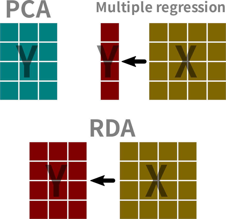
Redundancy Analysis

Greg Nishihara

2024 / 07 / 07

Redundancy Analysis

What is RDA

Redundancy analysis (RDA)¹ a canonical ordination² method and is one type of asymmetric canonical analysis³ that is used to analyze two data tables simultaneously. In RDA we are interested in how the environmental data $(\mathbf{X})$ influences ordination of the observation data $(\mathbf{Y})$. Recall that PCA is an unconstrained ordination⁴.

Asymmetric canonical analysis

RDA (Redundancy analysis)

Each canonical axis corresponds to a direction that is most related to linear combinations¹ of variables in $\mathbf{X}$.
Two ordinations
- Linear combinations of $\mathbf{Y}$.
- Linear combinations of $\mathbf{\hat{Y}}$.
Preserves the Euclidean distance² among objects.

CCA (Canonical correspondence analysis)³

Simlar to RDA, except CCA preserves the $\chi^2$ distance between objects

LDA (Linear discriminant analysis)⁴

$\mathbf{Y}$ is divided in to $k$ groups described by a factor.
Searches for the linear combinations in $\mathbf{X}$ that can explain the groups by maximizing the dispersion of the centroids of groups.

Approaches to analyze community data

Use DCA to choose RDA or CCA.

If the length of the first DCA axis > 4 use CCA.
If the length of the first DCA axis > 3 use RDA.
If the length is between 3 and 4, use either CCA or RDA.

If you transform the $\mathbf{Y}$,

Do not apply DCA.
Choose RDA for the analysis.

Use distance-based RDA.

RDA preparation

Each variable in $\mathbf{Y}$ and $\mathbf{X}$ should be centered (i.e., have means of zero).
Each variable in $\mathbf{Y}$ and $\mathbf{X}$ should be standardized (i.e., divide by the standard deviation).
Check for multi-collinearity among $\mathbf{X}$.

RDA Algorithm

Multiple regression $\mathbf{Y} \sim \mathbf{X}$
PCA on the expected value of $\mathbf{Y}$ determined from the multiple regression (i.e., $\mathbf{\hat{Y}}$)
PCA on the residuals of the multiple regression $\mathbf{Y_{res}} = \mathbf{Y} - \mathbf{\hat{Y}}$

Numerical examples

Observation data $(\mathbf{Y})$

The presence-absence community matrix¹ is a series of zeros and ones to indicate absence and presence, respectively.

The dimensions of the matrix (rows and columns).

seaweed |> dim()

[1] 147 108

Example of some data points.

seaweed[3:5, 3:5]

# A tibble: 3 × 3
  `Colpomenia-spp` `Dictyota-spiralis` `Gelidium-spp`
             <dbl>               <dbl>          <dbl>
1                0                   1              1
2                0                   0              1
3                0                   0              1

Hellinger transform

If we are interested in changes of relative species occurrence, then one good transformation is the Hellinger transform. The Hellinger transform is the square root of each element in a row divided by its row-sum.

\[ y\prime_{ij} = \sqrt{\frac{y_{ij}}{\sum y_{i}}} \]

Y = decostand(seaweed, "hellinger")

Y[3:5, 3:5]

  Colpomenia-spp Dictyota-spiralis Gelidium-spp
3              0         0.2294157    0.2294157
4              0         0.0000000    0.2182179
5              0         0.0000000    0.2182179

sqrt(seaweed[3:5, 3:5] / rowSums(seaweed)[3:5])

  Colpomenia-spp Dictyota-spiralis Gelidium-spp
1              0         0.2294157    0.2294157
2              0         0.0000000    0.2182179
3              0         0.0000000    0.2182179

Standardize environmental data

The environmental variables should be standardized (i.e, find the z-score).

\[ z = \frac{x - \bar{x}}{s} \] where $x$ is the value, $\bar{x}$ is the mean value of $x$, and $s$ is the standard deviation of $x$. This data is already standardized.

envdata |> print(n = 3)

# A tibble: 147 × 10
  year  season station month depth_mean pla_10…¹ sed_d…² herbi…³ compe…⁴ temp_…⁵
  <fct> <fct>  <fct>   <fct>      <dbl>    <dbl>   <dbl>   <dbl>   <dbl>   <dbl>
1 2021  WS     St01    4         -0.904   -1.34   -0.904   1.84   -0.372    1.92
2 2021  WS     St02    4         -0.254   -1.03   -0.783   0.122  -0.673    1.20
3 2021  WS     St03    4          1.88    -0.151  -0.213   0.837   1.50    -1.32
# … with 144 more rows, and abbreviated variable names ¹pla_100g_day_mean,
#   ²sed_day_mean, ³herbivorous_A_mean, ⁴competing_A_mean, ⁵temp_range_mean

Check length of first axis

If the length of the first axis is > 4.5, then use CCA not RDA (Leps & Smilauer 2003).

> 4 CCA: cca()
3 ~ 4: rda() or cca()
< 3 RDA: rda()

decorana(Y)


Call:
decorana(veg = Y) 

Detrended correspondence analysis with 26 segments.
Rescaling of axes with 4 iterations.
Total inertia (scaled Chi-square): 4.9589 

                       DCA1   DCA2   DCA3   DCA4
Eigenvalues          0.3195 0.2796 0.1848 0.1298
Additive Eigenvalues 0.3195 0.2797 0.1825 0.1250
Decorana values      0.3435 0.2744 0.1757 0.1325
Axis lengths         3.5600 2.9877 2.8427 2.1297

Note

If the Hellinger transform is applied, then it is simpler to use rda() and not worry about the dca().

Null Model

Define the null model and the full model of the multiple linear regression component.

nullmodel = Y ~ 1
fullmodel = Y ~ pla_100g_day_mean + 
  temp_range_mean +
  season + 
  competing_A_mean +
  herbivorous_A_mean +
  sed_day_mean +
  depth_mean

Forward selection

Use forward selection to eliminate unnecessary environmental variables. Removing variables will affect the scores and loadings.

Fit the null model.

rdamodel0 = rda(formula(nullmodel), data = envdata)

Fit the full model.

rdamodelf = rda(formula(fullmodel), data = envdata)

Run the forward selection.

rdamodel = ordiR2step(rdamodel0, # null
                     scope = formula(fullmodel), # full
                     R2permutations = 2^15,
                     trace = FALSE) # change to TRUE to see the selection process!

Results

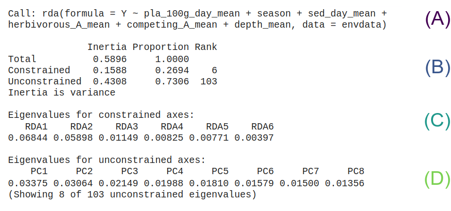
(A) RDA model selected by ordiR2step().

(B) The variance and proportions explained by the constrained and unconstrained parts of the model.

(D) The eigenvalues of the unconstrained components. These are the eigenvalues of the PCA run on the expected values.

Variance inflation factor

Use the variance inflation factor (VIF)¹ to check for multi-collinearity². If it is larger than 10, then variable is can be removed from the model.

vif.cca(rdamodel)

 pla_100g_day_mean           seasonWS       sed_day_mean herbivorous_A_mean 
          2.064950           1.024439           2.455251           3.070272 
  competing_A_mean         depth_mean 
          3.936895           3.396944

Redundancy analysis model

Solve for the eigenvalues $(\mathbf{\lambda_k})$ and eigenvectors $(\mathbf{u_k})$ of the redundancy analysis model.

\[ \left(\mathbf{S_{YX}}\mathbf{S_{XX}^{-1}}\mathbf{S_{YX}^\prime} - \mathbf{\lambda_k}\mathbf{I}\right)\mathbf{u_k}=0 \]

where, $\mathbf{S_{YX}}$ is the covariance matrix of $\mathbf{Y}$ and $\mathbf{Y}$, $\mathbf{S_{XX}^{-1}}$ is the covariance matrix of $, and $\mathbf{I}$ is the identity matrix.

Find the solution

First standardize the Y and X matrices.

Y = iris[, 1:2]
X = iris[, 3:4]
X = apply(X, 2, scale)
Y = apply(Y, 2, scale)

Next, fit the rda() version for comparison.

rdaout = rda(Y~X)

Then find $\mathbf{\hat{Y}}$ multivariate linear regression $\mathbf{Y} \sim \mathbf{X}$.

sxxinv = solve(t(X) %*% X)
syx = t(Y) %*% X
syxtr = t(syx)
Yhat = X %*% sxxinv %*% syxtr
Yres = Y - Yhat

Confirm the eigenvalues

Calculate the eigenvalues for the PCA part.

# PCA part
svd(Yres)$d^2 / (nrow(Y) -1)

[1] 0.8965380 0.1240973

rdaout$CA$eig

      PC1       PC2 
0.8965380 0.1240973

Calculate the eigenvalues for the RDA part.

# RDA part
svd(Yhat)$d^2 / (nrow(Y) - 1)

[1] 0.96547259 0.01389207

rdaout$CCA$eig

      RDA1       RDA2 
0.96547259 0.01389207

Confirm the eigenvectors

svd(Yres)$v

          [,1]       [,2]
[1,] 0.3767512  0.9263145
[2,] 0.9263145 -0.3767512

rdaout$CA$v

                   PC1        PC2
Sepal.Length 0.3767512  0.9263145
Sepal.Width  0.9263145 -0.3767512

svd(Yhat)$v

           [,1]      [,2]
[1,]  0.8891863 0.4575454
[2,] -0.4575454 0.8891863

rdaout$CCA$v

                   RDA1      RDA2
Sepal.Length  0.8891863 0.4575454
Sepal.Width  -0.4575454 0.8891863

Calcualte inertias

n = nrow(Y)
constrained = sum(svd(Yhat)$d^2 / (n - 1))
unconstrained = sum(svd(Yres)$d^2 / (n - 1))
total = constrained + unconstrained

tibble(type = c("Total", "Constrained", "Unconstrained"),
       Inertia = c(total, constrained, unconstrained)) |> 
  mutate(Proportion = Inertia / total)

# A tibble: 3 × 3
  type          Inertia Proportion
  <chr>           <dbl>      <dbl>
1 Total           2.00       1    
2 Constrained     0.979      0.490
3 Unconstrained   1.02       0.510

rdaout

Call: rda(formula = Y ~ X)

              Inertia Proportion Rank
Total          2.0000     1.0000     
Constrained    0.9794     0.4897    2
Unconstrained  1.0206     0.5103    2
Inertia is variance 

Eigenvalues for constrained axes:
  RDA1   RDA2 
0.9655 0.0139 

Eigenvalues for unconstrained axes:
   PC1    PC2 
0.8965 0.1241

Confirm the site scores

rdascores = scores(rdaout, scaling = 0, display = "sites") |> as_tibble()
eigscores = Y %*% svd(Yhat)$v %*% diag(1/svd(Yhat)$d)  |> as_tibble()
ggplot() + 
  geom_point(aes(x = V1, y = V2, color = "EIG"), data = eigscores, size = 3) +
  geom_point(aes(x = RDA1, y = RDA2, color = "RDA"), data = rdascores, size = 1) +
  scale_color_viridis_d(end = 0.8)

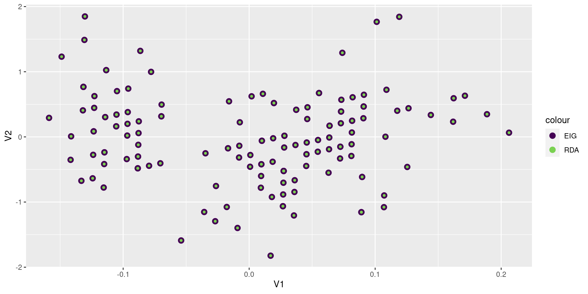
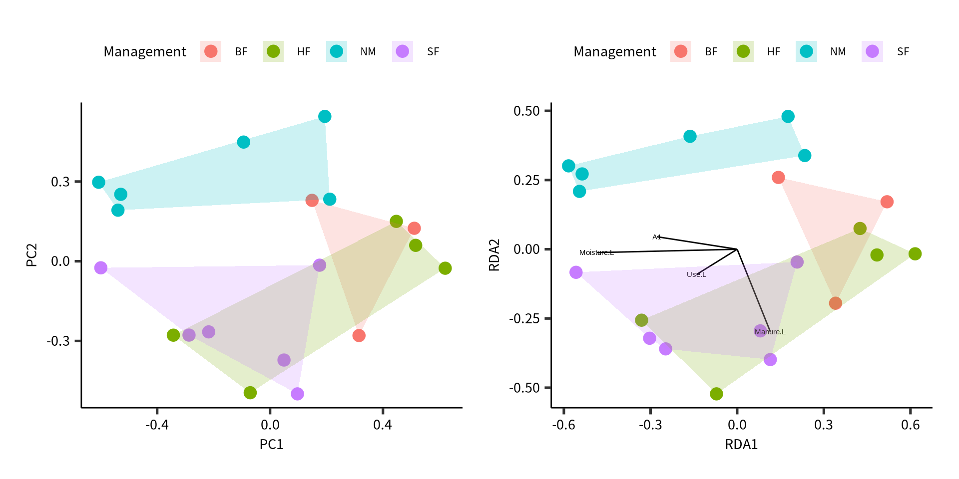
Confirm the environmental variables

variables = str_remove_all(colnames(Y), "[a-z|\\.]")
rdavariables = scores(rdaout, scaling = 0, display = "bp") |> as_tibble()
temp = t(X) %*% svd(Yhat)$u
svdvariables = apply(temp, 1, \(x) x / sqrt(sum(x^2))) |> t() |> as_tibble()
rdavariables = rdavariables |> mutate(variables = variables, .before = 1)
svdvariables = svdvariables |> mutate(variables = variables, .before = 1)
full_join(rdavariables, svdvariables, by = "variables")

# A tibble: 2 × 5
  variables  RDA1  RDA2    V1    V2
  <chr>     <dbl> <dbl> <dbl> <dbl>
1 SL        0.988 0.152 0.988 0.152
2 SW        0.911 0.413 0.911 0.413

Example analysis

Example data set.

Dune meadow vegetation data.

A1 soil thickness
Moisture ordered factor of levels 1 < 2 < 4 < 5
Management factor of 4 levels
Use ordered factor Hayfield < Haypastu < Pasture
Manure Ordered factor 0 < 1 < 2 < 3 < 4

   Achimill Agrostol Airaprae Alopgeni Anthodor Bellpere Bromhord Chenalbu
1         1        0        0        0        0        0        0        0
2         1        0        0        1        0        1        1        0
3         0        1        0        1        0        1        0        0
4         0        1        0        1        0        1        1        0
5         1        0        0        0        1        1        1        0
6         1        0        0        0        1        0        0        0
7         1        0        0        0        1        0        1        0
8         0        1        0        1        0        0        0        0
9         0        1        0        1        0        0        0        0
10        1        0        0        0        1        1        1        0
11        0        0        0        0        0        0        0        0
12        0        1        0        1        0        0        0        0
13        0        1        0        1        0        0        0        1
14        0        1        0        0        0        0        0        0
15        0        1        0        0        0        0        0        0
16        0        1        0        1        0        0        0        0
17        1        0        1        0        1        0        0        0
18        0        0        0        0        0        1        0        0
19        0        0        1        0        1        0        0        0
20        0        1        0        0        0        0        0        0
   Cirsarve Comapalu Eleopalu Elymrepe Empenigr Hyporadi Juncarti Juncbufo
1         0        0        0        1        0        0        0        0
2         0        0        0        1        0        0        0        0
3         0        0        0        1        0        0        0        0
4         1        0        0        1        0        0        0        0
5         0        0        0        1        0        0        0        0
6         0        0        0        0        0        0        0        0
7         0        0        0        0        0        0        0        1
8         0        0        1        0        0        0        1        0
9         0        0        0        1        0        0        1        1
10        0        0        0        0        0        0        0        0
11        0        0        0        0        0        1        0        0
12        0        0        0        0        0        0        0        1
13        0        0        0        0        0        0        0        1
14        0        1        1        0        0        0        0        0
15        0        1        1        0        0        0        1        0
16        0        0        1        0        0        0        1        0
17        0        0        0        0        0        1        0        0
18        0        0        0        0        0        0        0        0
19        0        0        0        0        1        1        0        0
20        0        0        1        0        0        0        1        0
   Lolipere Planlanc Poaprat Poatriv Ranuflam Rumeacet Sagiproc Salirepe
1         1        0       1       1        0        0        0        0
2         1        0       1       1        0        0        0        0
3         1        0       1       1        0        0        0        0
4         1        0       1       1        0        0        1        0
5         1        1       1       1        0        1        0        0
6         1        1       1       1        0        1        0        0
7         1        1       1       1        0        1        0        0
8         1        0       1       1        1        0        1        0
9         1        0       1       1        0        1        1        0
10        1        1       1       1        0        0        0        0
11        1        1       1       0        0        0        1        0
12        0        0       0       1        0        1        1        0
13        0        0       1       1        1        0        1        0
14        0        0       0       0        1        0        0        0
15        0        0       0       0        1        0        0        0
16        0        0       0       1        1        0        0        0
17        0        1       1       0        0        0        0        0
18        1        1       1       0        0        0        0        1
19        0        0       0       0        0        0        1        1
20        0        0       0       0        1        0        0        1
   Scorautu Trifprat Trifrepe Vicilath Bracruta Callcusp
1         0        0        0        0        0        0
2         1        0        1        0        0        0
3         1        0        1        0        1        0
4         1        0        1        0        1        0
5         1        1        1        0        1        0
6         1        1        1        0        1        0
7         1        1        1        0        1        0
8         1        0        1        0        1        0
9         1        0        1        0        1        0
10        1        0        1        1        1        0
11        1        0        1        1        1        0
12        1        0        1        0        1        0
13        1        0        1        0        0        0
14        1        0        1        0        0        1
15        1        0        1        0        1        0
16        0        0        0        0        1        1
17        1        0        0        0        0        0
18        1        0        1        1        1        0
19        1        0        1        0        1        0
20        1        0        0        0        1        1

     A1 Moisture Management      Use Manure
1   2.8        1         SF Haypastu      4
2   3.5        1         BF Haypastu      2
3   4.3        2         SF Haypastu      4
4   4.2        2         SF Haypastu      4
5   6.3        1         HF Hayfield      2
6   4.3        1         HF Haypastu      2
7   2.8        1         HF  Pasture      3
8   4.2        5         HF  Pasture      3
9   3.7        4         HF Hayfield      1
10  3.3        2         BF Hayfield      1
11  3.5        1         BF  Pasture      1
12  5.8        4         SF Haypastu      2
13  6.0        5         SF Haypastu      3
14  9.3        5         NM  Pasture      0
15 11.5        5         NM Haypastu      0
16  5.7        5         SF  Pasture      3
17  4.0        2         NM Hayfield      0
18  4.6        1         NM Hayfield      0
19  3.7        5         NM Hayfield      0
20  3.5        5         NM Hayfield      0

# A tibble: 20 × 5
      A1 Moisture Management Use      Manure
   <dbl> <ord>    <fct>      <ord>    <ord> 
 1   2.8 1        SF         Haypastu 4     
 2   3.5 1        BF         Haypastu 2     
 3   4.3 2        SF         Haypastu 4     
 4   4.2 2        SF         Haypastu 4     
 5   6.3 1        HF         Hayfield 2     
 6   4.3 1        HF         Haypastu 2     
 7   2.8 1        HF         Pasture  3     
 8   4.2 5        HF         Pasture  3     
 9   3.7 4        HF         Hayfield 1     
10   3.3 2        BF         Hayfield 1     
11   3.5 1        BF         Pasture  1     
12   5.8 4        SF         Haypastu 2     
13   6   5        SF         Haypastu 3     
14   9.3 5        NM         Pasture  0     
15  11.5 5        NM         Haypastu 0     
16   5.7 5        SF         Pasture  3     
17   4   2        NM         Hayfield 0     
18   4.6 1        NM         Hayfield 0     
19   3.7 5        NM         Hayfield 0     
20   3.5 5        NM         Hayfield 0


Call:
rda(formula = dune ~ A1 + Moisture + Use + Manure, data = dune.env) 

Partitioning of variance:
              Inertia Proportion
Total           5.261     1.0000
Constrained     3.384     0.6432
Unconstrained   1.877     0.3568

Eigenvalues, and their contribution to the variance 

Importance of components:
                        RDA1   RDA2    RDA3    RDA4    RDA5    RDA6    RDA7
Eigenvalue            1.4129 0.7859 0.28559 0.24176 0.17851 0.15076 0.12636
Proportion Explained  0.2686 0.1494 0.05429 0.04596 0.03393 0.02866 0.02402
Cumulative Proportion 0.2686 0.4180 0.47226 0.51822 0.55215 0.58081 0.60483
                        RDA8    RDA9    RDA10     PC1     PC2     PC3     PC4
Eigenvalue            0.1021 0.06278 0.037263 0.43922 0.43799 0.29683 0.22855
Proportion Explained  0.0194 0.01193 0.007083 0.08349 0.08326 0.05643 0.04345
Cumulative Proportion 0.6242 0.63616 0.643248 0.72674 0.81000 0.86643 0.90988
                          PC5     PC6     PC7     PC8      PC9
Eigenvalue            0.16015 0.12726 0.09615 0.06368 0.026875
Proportion Explained  0.03044 0.02419 0.01828 0.01210 0.005109
Cumulative Proportion 0.94032 0.96451 0.98279 0.99489 1.000000

Accumulated constrained eigenvalues
Importance of components:
                        RDA1   RDA2   RDA3    RDA4    RDA5    RDA6    RDA7
Eigenvalue            1.4129 0.7859 0.2856 0.24176 0.17851 0.15076 0.12636
Proportion Explained  0.4175 0.2322 0.0844 0.07144 0.05275 0.04455 0.03734
Cumulative Proportion 0.4175 0.6498 0.7342 0.80563 0.85838 0.90293 0.94027
                         RDA8    RDA9   RDA10
Eigenvalue            0.10206 0.06278 0.03726
Proportion Explained  0.03016 0.01855 0.01101
Cumulative Proportion 0.97043 0.98899 1.00000

Scaling 2 for species and site scores
* Species are scaled proportional to eigenvalues
* Sites are unscaled: weighted dispersion equal on all dimensions
* General scaling constant of scores:

Permutation test for rda under reduced model
Terms added sequentially (first to last)
Permutation: free
Number of permutations: 999

Model: rda(formula = dune ~ A1 + Moisture + Use + Manure, data = dune.env)
         Df Variance      F Pr(>F)   
A1        1  0.54865 2.6311  0.006 **
Moisture  3  1.44897 2.3162  0.002 **
Use       2  0.50253 1.2050  0.257   
Manure    4  0.88368 1.0595  0.406   
Residual  9  1.87670                 
---
Signif. codes:  0 '***' 0.001 '**' 0.01 '*' 0.05 '.' 0.1 ' ' 1

Permutation test for rda under reduced model
Forward tests for axes
Permutation: free
Number of permutations: 999

Model: rda(formula = dune ~ A1 + Moisture + Use + Manure, data = dune.env)
         Df Variance      F Pr(>F)   
RDA1      1  1.41288 6.7757  0.002 **
RDA2      1  0.78586 3.7687  0.117   
RDA3      1  0.28559 1.3696  0.996   
RDA4      1  0.24176 1.1594  1.000   
RDA5      1  0.17851 0.8561  0.999   
RDA6      1  0.15076 0.7230  1.000   
RDA7      1  0.12636 0.6060  1.000   
RDA8      1  0.10206 0.4894  1.000   
RDA9      1  0.06278 0.3011  1.000   
RDA10     1  0.03726 0.1787  0.999   
Residual  9  1.87670                 
---
Signif. codes:  0 '***' 0.001 '**' 0.01 '*' 0.05 '.' 0.1 ' ' 1

Redundancy Analysis

Redundancy Analysis

What is RDA

Asymmetric canonical analysis

Approaches to analyze community data

RDA preparation

RDA Algorithm

Numerical examples

Observation data \((\mathbf{Y})\)

Hellinger transform

Standardize environmental data

Check length of first axis

Null Model

Forward selection

Results

Variance inflation factor

Redundancy analysis model

Find the solution

Confirm the eigenvalues

Confirm the eigenvectors

Calcualte inertias

Confirm the site scores

Confirm the environmental variables

Example analysis