Comparing two groups

t 検定の紹介

Greg Nishihara

2024-07-07

A juvenile Sargassum macrocarpum

A random sample

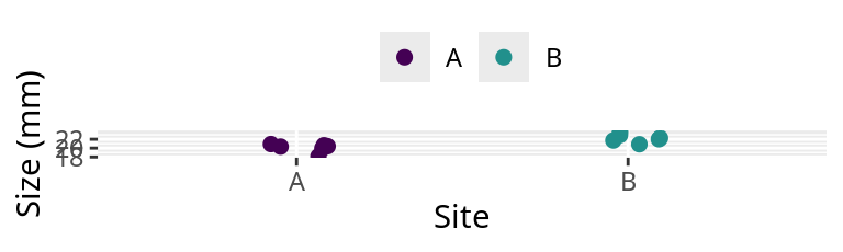
Table 1: Size (mm) of juvenile Sargassum macrocarpum（ノコギリモク）.

The table shows two groups of 6 juvenile Sargassum macrocarpum (ノコギリモク) that were sampled randomly. The two groups of juveniles are from two sites, A and B.

Each sample is given an sample I.D. of 1 to 6.

These data were generated with the R function with a true mean (\(\mu\)) of 20 and 22 for site A and B, respectively. The true standard deviation (\(\sigma\)) is 1 and 1 for site A and B, respectively.

Let’s compare the two groups

The mean (\(\overline{x}\)), standard deviation (\(s\)), and the standard error (s.e.) for juvenile S. macrocarpum from site A and B are:

• \(\overline{x}_A=\) 20.033, \(s_A=\) 1.003, and s.e. = 0.41
• \(\overline{x}_B=\) 22.25 and \(s_B=\) 0.971, and s.e. = 0.396

What is our question?

• If we want to statistically compare the size from the two sites, we need a question (i.e., a working hypothesis).

Working hypothesis (作業仮設): The size (width) of juvenile S. macrocarpum collected from site A and B are different.

• We know that the means for site A and B are different, but the standard deviations and standard errors are similar.
  • \(\overline{x}_A=\) 20.033; \(s=\) 1.003; s.e. = 0.41
  • \(\overline{x}_B=\) 22.25; \(s=\) 0.971; s.e. = 0.396

Define our hypotheses

Let’s formally define our statistical hypotheses.

• \(H_0\) (null hypothesis 帰無仮説): There is no difference in the paired values.

• \(H_A\) (alternative hypothesis 対立仮設): There is a difference in the paired values.

Other alternative hypotheses

• \(H_P\) (alternative hypothesis): The difference in paired values is positive.
• \(H_N\) (alternative hypothesis): The difference in paired values is negative.

Important: We can define an infinite number of hypotheses.

The most common alternative hypothesis is a test for an effect. For example, \(H_0\): there is no effect. \(H_A\): There is an effect.

Note: hypotheses is the plural form (複数形) of hypothesis.

Calculate the size differences among pairs

Assume that we can compare the paired differences (e.g., \(x_{A,1} - x_{B,1}\), \(x_{A,2} - x_{B,2}\), \(x_{A,3} - x_{B,3}\), \(\cdots\), \(x_{A,6} - x_{B,6}\)).

Recall the hypotheses

The two statistical hypotheses that we defined were:

• \(H_0\): There is no difference in the paired values.
• \(H_A\): There is a difference in the paired values.

The mean difference (\(\overline{x}_{A-B}\)) is -2.217, the standard deviation (\(s_{A-B}\)) is 1.289, and the standard error (\(\text{s.e.}_{A-B}\)) is 0.526

Note: The true difference \(\mu_{A-B}\) is -2, the true standard deviation \(\sigma_A = \sigma_B\) is 1.

If the samples can be paired, then the differences between site A and B are easy to determine.

Therefore, it is easy to calculate the mean, standard deviation, and standard error.

\[ \begin{aligned} \overline{x} &= \frac{1}{n}\sum x \qquad \text{mean} \\ s &= \sqrt{\frac{1}{n-1} \sum \left(x-\overline{x}\right)^2} \qquad \text{standard deviation} \\ \text{s.e.} &= \frac{s}{\sqrt{n}} \qquad \text{standard error of the} \end{aligned} \]

How do we statistically test if the differences are significant?

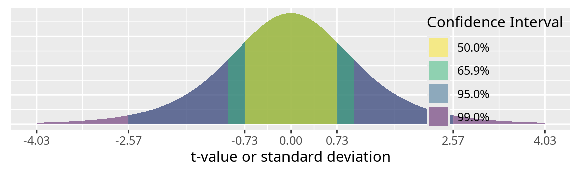
Distribution of the mean

Recall that the central limit theorem (中心極限定理) states that the distribution of the mean has a Gaussian (normal) distribution (正規分布).

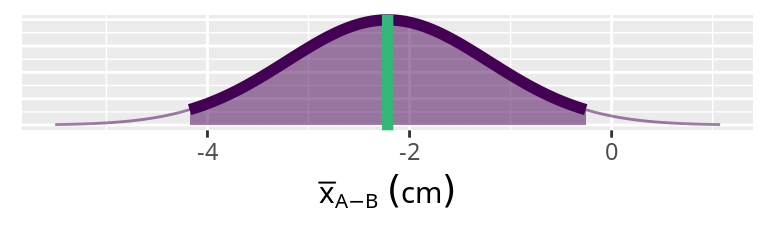
• \(\overline{x}_{A-B} =\) -2.217 (mean)
• \(s_{A-B}=\) 1.289 (standard deviation)
• s.e._A-B = 0.526 (standard error)

The shaded area is the 95% probability region. The width of the shaded area is called a confidence interval (信頼区間). If the significance level (有意水準) is \(\alpha = 0.05\), then the confidence interval is called a 95% confidence interval (95% 信頼区間).

The green vertical line is the sample mean (\(\overline{x}\)).

The thick line and the shaded region indicates the 95% confidence interval of the sample mean.

The thin line indicates a Gaussian distribution with a sample mean of -2.217.

The standard deviation is 0.526, which is the standard error of the mean.

We use the standard error because we are interested in the distribution of the mean values. If we were interested in the distribution of the observations, then we would use the standard deviation.

Since the value of zero is not included in the 95% confidence interval, we can reject the null hypothesis that \(\overline{x}_A = \overline{x}_B\) or \(x_{A-B}=0\).

So what is a confidence interval (信頼区間)?

Developing the confidence interval

The confidence interval is an interval \([l, u]\) with a lower bound of \(l\) and an upper bound of \(u\).

For a probability \(1-\alpha\), the interval \([l, u]\) for \(x\) is

\[ P(l \le x \le u) = 1-\alpha \] If \(\overline{x}\) is a sample mean, then the z-score (z値) is

\[ z = \frac{\overline{x}-\mu}{\sigma} \]

where \(\mu\) is the population mean and \(\sigma\) is the population standard deviation. Then, to find \(l\) and \(u\), we need to solve

\[ P(l \le z \le u) = 1-\alpha \]

for the interval \([l, u]\) of \(z\) given a probability of \(1-\alpha\).

Central limit theorem (中心極限定理)

Recall that the central limit theorem states that:

\[ \lim_{n\rightarrow\infty} \sqrt{n}\overbrace{\left(\frac{\overline{x}_n-\mu}{\sigma}\right)}^{z} \xrightarrow{d} N(0, 1) \]

Therefore, for \(\alpha = 0.05\), we can define an \([l, u]\)

\[ P\left(l \le z \le u \right) = 1-0.05 = 0.95 \]

For the standard normal distribution (\(N(0,1)\))

• \(l\) is the \(\alpha/2=0.05/2=0.025\) quantile.
• \(u\) is the \(1-\alpha/2=1-0.05/2=0.975\) quantile.

The z-score appears in the definition of the central limit theorem.

\[ z = \frac{\overline{x}-\mu}{\sigma} \]

As the number of samples increase, the distribution of \(\sqrt{n}\left(\frac{\overline{x}_n-\mu}{\sigma}\right)\) converges to a standard normal distribution.

The symbol \(\xrightarrow{d}\) in the model means, “converges in distribution.”

There are many different types of intervals.

• range (レンジ・範囲)
• prediction interval (予測区間)
• credible interval (信用区間)

The confidence interval provides information about the precision of our estimate of the mean.

The confidence interval is also a range of observations defined by the quantile of a distribution. For the mean values, a normal distribution is usually assumed because mean values follow the central limit theorem.

How do we find the \(l\) and \(u\) quantiles?

Determining the lower and upper quantiles of \(N(0, 1)\)

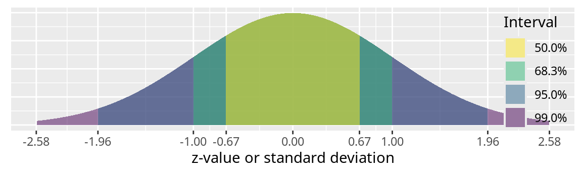
Note that \([-1 s, 1 s]\) is the 68.3% interval, \([-2 s, 2 s]\) is the 95.4% interval, and \([-3 s, 3 s]\) is the 99.7% interval.

The 50%, 68.3%, 95%, and 99% confidence intervals are indicated by the shaded region.

The shaded area indicates the probability.

Along the x-axis are the z-scores or a multiple of the standard deviation.

Table of quantiles for \(N(0, 1)\)

Significance level, α	Confidence interval (%)	± quantile
0.500	50.000	0.674
0.317	68.269	1.000
0.200	80.000	1.282
0.100	90.000	1.645
0.050	95.000	1.960
0.046	95.450	2.000
0.025	97.500	2.241
0.003	99.730	3.000
0.000	99.994	4.000

Calculating the confidence interval

Let \(x = \overline{x}_{A-B} =\) -2.217, \(s = \text{s.e.} =\) 0.526, \(\sigma_A = \sigma_B =\) 1, and and \(\alpha = 0.05\).

\[ P\left(l \le \frac{\overline{x}-\mu}{\sigma}\le u\right) = 1-\alpha = 0.95 \]

\[ P\left(\overline{x} +l \sigma \le \mu \le \overline{x} + u\sigma\right) = 1-\alpha = 0.95 \]

When \(\alpha= 0.05\), the \(l\) and \(u\) quantiles are \(l=\) -1.96 and \(u=\) 1.96, and \(\sigma = 1\).

\[ P( -2.217 + -1.96 \times 1 \le x \le -2.217 + 1.96 \times 1 ) \]

\[ P( -4.177 \le x \le -0.257 ) = 0.95 \]

The 95% confidence interval of \(\overline{x}=\) -2.217 is \([-4.177, -0.257 ]\).

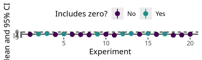
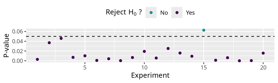
Confidence intervals for each experiment when \(\sigma\) is known

\(\sigma_A = \sigma_B=\) 1, \(H_0:\) \(\overline{x}_A = \overline{x}_B\) or \(\overline{x}_{A-B}=0\)

How often does the confidence interval contain 0?

• The true difference is -2, therefore \(H_0\) is false.
• If we do not reject \(H_0\), we are making a Type-II Error (第2種の誤り).
• The 95% confidence intervals of 8 experiments include 0.
• The error rate is \(\beta=\) 8 / 20 = 0.4 or 40%.
• The power of this analysis (\(1 - \beta\)) is 0.6

We made some wrong assumptions

The z-score when population mean \(\mu\) and population standard deviation \(\sigma\) is known follows a standard normal distribution.

\[ z = \frac{\overline{x} - \mu}{\sigma}\sim N(0,1) \] However, if you do not know the population standard deviation, we must calculate the t-value.

\[ t_{\overline{x}} = \frac{\overline{x} - x_0}{s.e.} = \frac{\overline{x} - x_0}{s / \sqrt{n}} \]

Which follows a t-distribution. \(x_0\) is a constant, and is often set to zero.

Determining the lower and upper quantiles of \(t(d.f.)\)?

Note that the degrees-of-freedom (d.f., 自由度) for the t-distribution is \(N -1\) = 5.

Table of quantiles for \(t(d.f. = 5)\)

Quantiles of the t distribution for d.f. = 5.

Significance level, \(\alpha\)	Confidence interval (%)	\(\pm\) quantile
0.500	50.000	0.727
0.363	63.678	1.000
0.200	80.000	1.476
0.102	89.806	2.000
0.100	90.000	2.015
0.050	95.000	2.571
0.030	96.990	3.000
0.025	97.500	3.163
0.010	98.968	4.000

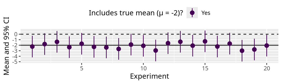
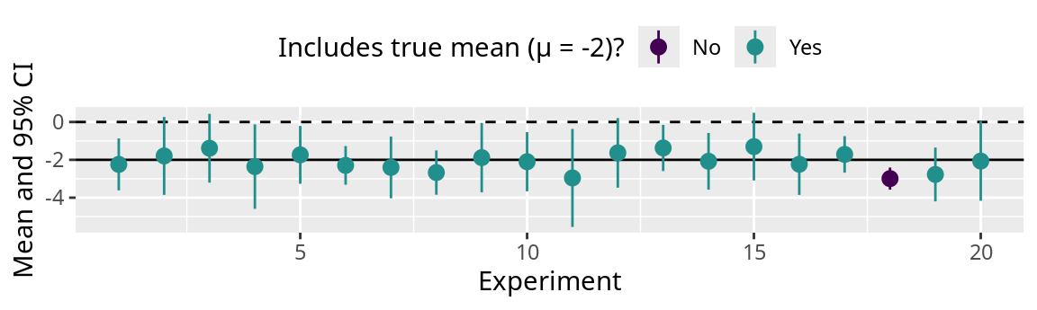
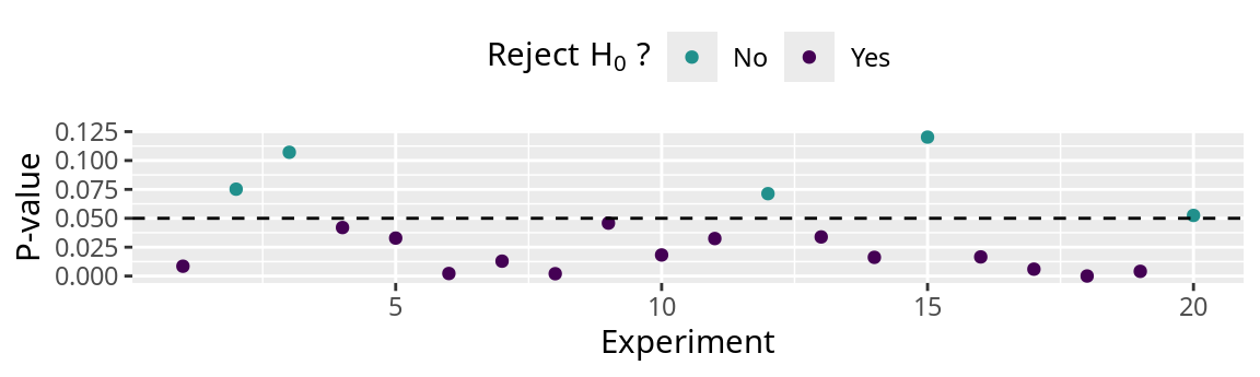
Confidence intervals for each experiment when \(\sigma\) is unknown

\(H_0:\) \(\overline{x}_A = \overline{x}_B\) or \(\overline{x}_{A-B}=0\)

This figure shows 20 sample means and their confidence intervals. The dashed horizontal line indicates zero and the solid horizontal line indicates the true difference 0.

The dots indicate the sample mean and the vertical lines indicate the range of the 95% confidence interval.

The green symbols indicates that the interval includes the true mean.

Out of 20 trials, the 95% confidence included the true difference 19 times.

What does the confidence interval mean?

A 95% confidence interval implies that after 100 experiments, about 95 of the confidence intervals will include the true mean.

• It does not mean that the true mean is in the interval.
• It does not mean that there is a 95% chance that the true mean in in the interval, since the size of the confidence interval varies with the sample.
• It also does not mean that there is a 95% chance that the mean of the next experiment will be in the confidence interval.

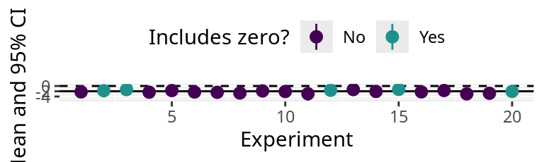
How often does the confidence interval contain 0?

• The true difference is -2, therefore \(H_0\) is false.
• If we do not reject \(H_0\), we are making a Type-II Error (第2種の誤り).
• The 95% confidence intervals of 5 experiments include 0. So for 5 experiments, we do not reject \(H_0\).
• The error rate is \(\beta=\) 5 / 20 = 0.25 or 25%.
• The power of this analysis (\(1 - \beta\)) is 0.75

These are informal ways of testing differences, howerver in practice we use more sophisticated formalized methods.

Formal tests of group means

The paired t-test

Type-II error rate \(\beta\) = 5 / 20 = 25% and power (\(1-\beta\)) is 0.75.

t-test (unpaired assuming unequal variance)

Type-II error rate \(\beta\) = 1 / 20 = 5% and power (\(1-\beta\)) is 0.95.

The null hypothesis of the t-test

\(H_0\) null hypothesis (帰無仮説): \(\overline{x}_A - \overline{x}_B = \overline{x}_{A-B}=0\)

Paired t-test

Paired t-test (対応ありのt検定)

We need to calculate the t-value, which is the statistic for the t-test.

\[ t^* = \frac{\overline{x}_{A-B} - \mu}{s_{A-B} / \sqrt{n}} \]

And determine the degrees-of-freedom (自由度) which is \(n-1\).

Used when observations can be paired. For example the length of the left and right fin of a fish.

Independent two sample t-test

There are two versions.

Equal variance (等分散)

\[ t^* = \frac{\overline{x}_A - \overline{x}_B}{s_p \sqrt{1 / n_A + 1/n_B}} \] \[ s_p = \sqrt{ \frac{(n_A-1)s_A^2 + (n_B-1)s_B^2} {n_A + n_B -2}} \] Degrees-of-freedom is \(n_A + n_B - 2\).

Unequal variance, Welch’s t-test (ウェルチのt検定)

\[ t^* = \frac{\overline{x}_A - \overline{x}_B}{s_p} \]

\[ s_p = \sqrt{ \frac{s_A^2}{n_A} + \frac{s_B^2}{n_B}} \] Degrees-of-freedom is calculated with the Welch-Satterthwaite Equation.

\(s\) is the sample standard deviation. \(n\) is the number of samples. \(\overline{x}\) is the mean. \(t^*\) is the t-value.

Welch-Satterthwaite Equation

\[ \text{degrees-of-freedom} = \frac{ \left(\frac{s_A^2}{n_A} + \frac{s_B^2}{n_B}\right)^2 } {\frac{\left(s_A^2 / n_A\right)^2}{n_A-1} + \frac{\left(s_B^2 / n_B\right)^2}{n_B-1}} \]

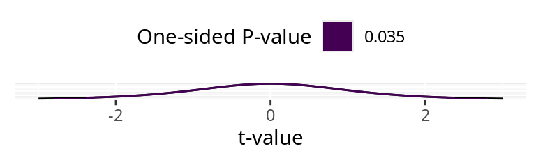
The unpaired t-test

\[ \begin{aligned} t^* &= \frac{\overline{x}_{A-B} - \mu}{s_{A-B} / \sqrt{n}} \\ t^* &= \frac{-2.467}{2.642 / \sqrt{6}} \\ t^* &= -2.287 \end{aligned} \]

• \(\overline{x}_{A-B}=\) -2.467
• \(\mu=0\)
• \(n\) = 6
• \(s_{A-B}=\) 2.642

• \(\alpha\) = 0.05
• t-value: -2.287
• One-sided P-value: 0.035
• Two-sided P-value: 0.071

The juvenile S. macrocarpum size observations cannot be paired, so this is the wrong test.

The correct test is Welch’s t-test

\[ \begin{aligned} t^* &= \frac{\overline{x}_A -\overline{x}_B}{s_p} \\ s_p &= \sqrt{\frac{s_A^2}{n_A} + \frac{s_B^2}{n_B}} \\ s_p &= \sqrt{\frac{1.995^2}{6} + \frac{1.961^2}{6}} \\ t^* &= \frac{10.05 - 12.517}{1.142} \\ t^* &= -2.16 \\ \text{d.f.} &= 9.997 \end{aligned} \]

• \(\alpha\) = 0.05
• t-value: -2.16
• One-sided P-value: 0.028
• Two-sided P-value: 0.056

The P-value decreases, but \(0.056 \ge \alpha= 0.05\). We can’t reject \(H_0\).

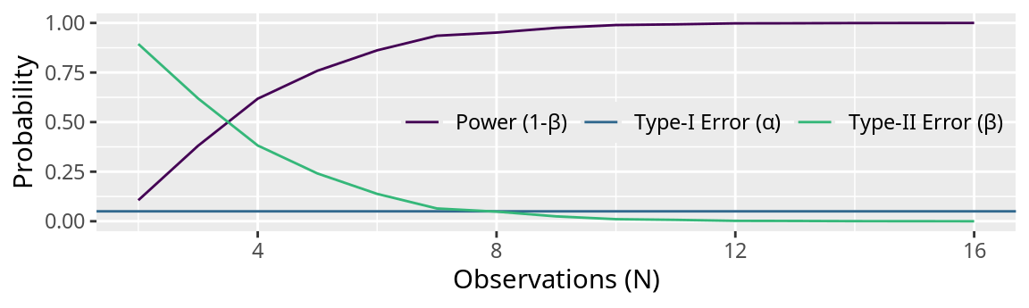
Behavior of the t-test (equal variance)

Increasing the number of observations decrease the Type-II error rate and increases the power of the test. The Type-I error rate is fixed at \(\alpha=0.05\).

The true mean (\(\mu\)) is for site A and B is 20 and 22, respectively. The true standard deviation (\(\sigma\)) for site A and B is 1 and 1, respectively.

For each sample size of {2, 3, 4, 5, 6, 7, 8, 9, 10, 11, 12, 13, 142, 3, 4, 5, 6, 7, 8, 9, 10, 11, 12, 13, 14, and 16} a total of 2000 simulated samples were created.

When the sample size (\(N\)) is small, the Type-II error rate is high and the power of the t-test is low.

Increasing the sample size increases the power of the t-test and decreases the Type-II error rate.

When the \(N\) = 6, the Type-II error rate is 0.138 and the power of the t-test is 0.862.

When the \(N\) = 10, the Type-II error rate is 0.011 and the power of the t-test is 0.99.

The Type-I error rate is predefined and does not change with the number of observations.

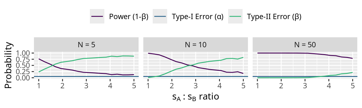
Behavior of the t-test (unequal variance)

Unbalanced variances (\(s^2\)) increase the risk of a Type-II error rate (\(\beta\)) and decrease the power (\(1-\beta\)) of the t-test. The Type-I error rate is fixed at \(\alpha=0.05\).

The true mean (\(\mu\)) is for site A and B is 20 and 22, respectively. The true standard deviation (\(\sigma\)) for site A is 1 and for site B is \(k\times\sigma_B\), respectively. \(k\) is a multiplier.

When the standard deviations (variances) are not equal, the Type-II error rate and power of the t-test varies.

When \(s_A / s_B \rightarrow\infty\), the Type-II error rate increases and the power decreases.

When the sample size is high, the t-test is less sensitive to unequal variances.

The Type-I error rate is predefined and does not change with the number of observations.

Welch’s t-test R code

• Code
• Output

library(tidyverse)
A = c(9.8,11.1,10.7,10.7,11.8,6.2)
B = c(12.5,13.8,12.0,15.5,9.8,11.5)
data = tibble(A, B)
data = data %>% pivot_longer(cols = c(A,B))
t.test(value ~ name, data = data) # ウェルチ t 検定
# t.test(A, B) # Alternative method

# two-sample, equal variance t-test (等分散 t 検定)
# t.test(value ~ name, data = data, var.equal = TRUE) 

Welch’s t-test does not require equal variances or equal sample size.

The two-sample t-test requires equal variances.

    Welch Two Sample t-test

data:  value by name
t = -2.16, df = 9.9971, p-value = 0.05612
alternative hypothesis: true difference in means between group A and group B is not equal to 0
95 percent confidence interval:
 -5.01124979  0.07791646
sample estimates:
mean in group A mean in group B 
       10.05000        12.51667