16 Wavelet 解析

16.1 必要なパッケージ

library(tidyverse)
library(lubridate)
library(gnnlab)
library(furrr)
library(biwavelet)

ウェーブレット変換は時系列データから時間的変化の特徴と周波数成分を調べるために使います。 細かい説明はいつか追加します。 本章を完成するまでは、次の論文を参考にしてください。

Cazelles B., Chavez M., Berteaux D., Menard F., Vik J.O., Jenouvrier S., and Stenseth N.C. 2008. Wavelet analysis of ecological time series. Oecologia 156: 287-304.

Grinsted A., Moore J.C., and Jevrejeva S. 2004. Application of the cross wavelet transform and wavelet coherence to geophysical time series. Nonlinear Processes in Geophysics 11: 561-566.

Torrence C. and Compo G.P. 1998. A practical guide to wavelet analysis. Bulletin of the American Meteorological Society 79: 61-78.

Torrence C and Webster P.J. 1998. The annual cycle of persistence in the El Nino/Southern Oscillation. Quarterly Journal of the Royal Meteorological Society 124: 1985-2004.

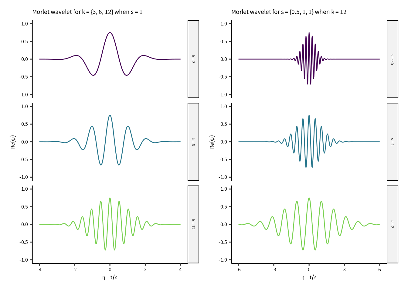
\[ \psi(\eta) = \frac{1}{\sqrt[\leftroot{-2}\uproot{3}4]{\pi}}\;e^{\eta^2/2}\;e^{ik\eta} \] パラメータ $\eta$ は時間 $(t)$ とウェーブレットスケール $(s)$ の比率です。ウェーブレットスケールを下げると時間軸方向の分解能が上がります。ウェーブレットパラメータ $k$ はモレー・ウェーブレットの振動数（山の数）を制御しています。よって、$k$ を上げると、周波数分解能が上がります。

では、biwavelet パッケージで次の波形を解析してみましょう。

\[ \begin{aligned} y &= \sin(2 \pi \omega) \\ \omega &= 50 t^2 + 10 \end{aligned} \] この波形の角周波数 $(\omega)$ は徐々に高くなります。

ft = function(t) {
  f = 50 * t^2 + 10
  sin(2 * pi * f )
}
z = tibble(t = seq(0, 1, length = 3000)) |> mutate(y = ft(t))

ggplot(z) + geom_line(aes(x = t, y = y)) +
  scale_x_continuous("t") +
  scale_y_continuous("y")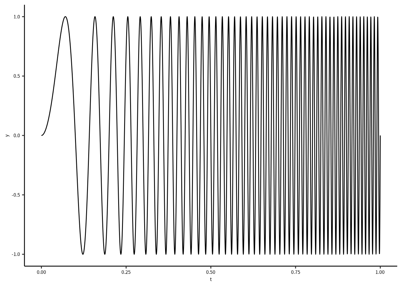

biwavelet の wt() 関数でウェーブレット解析をします。 wt() に渡すデータは行列としてわたしましょう。行列の1列目には時間情報、2列名には解析したい値です。

wtout = wt(as.matrix(z), mother = "morlet")

plot(wtout)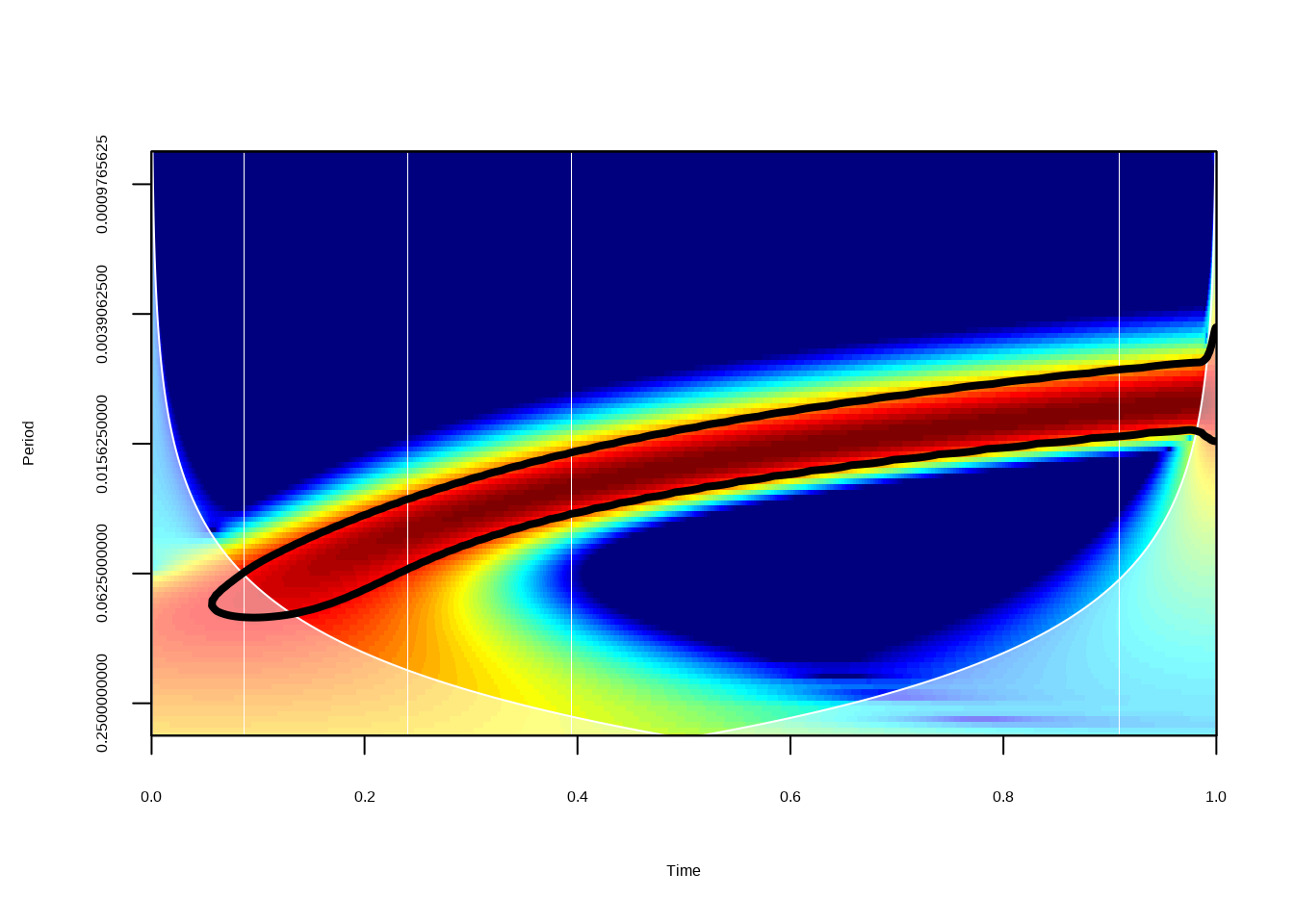

$これはウェーブレット解析のパワーを示す図です。パワーの低いところは青色、パワーの高いところは赤色です。黒線は統計学的に優位な領域を示しています。赤色の部分が時間につれ、周期が上昇しています。ウェーブレット解析で角周波数の傾向を十分抽出できたとおもいます。白くなっているところは cone of influence (COI) です。 COIは解析アルゴリズムの精度が落ちているところを示しているので、示されたパワーは両端から $e^{-2}$ に従って下がります。$

Figure 16.1: これはウェーブレット解析のパワーを示す図です。パワーの低いところは青色、パワーの高いところは赤色です。黒線は統計学的に優位な領域を示しています。赤色の部分が時間につれ、周期が上昇しています。ウェーブレット解析で角周波数の傾向を十分抽出できたとおもいます。白くなっているところは cone of influence (COI) です。 COIは解析アルゴリズムの精度が落ちているところを示しているので、示されたパワーは両端から $e^{-2}$ に従って下がります。

16.2 解析に使う関数

Wavelet を求めるための関数です。コアは biwavelet パッケージの wt() 関数です。マザー・ウェーブレット (mother wavelet) はモレーウェーブレット (Morlet wavelet) に固定しています。 wt() には DoG (derivative of gaussian) と Paul ウェーブレットも使えます。

calculate_wavelet = function(df, obs, tau = NULL, fs = 6, dB = TRUE) {
  pad_cname = function(x, w) {
    x = str_pad(x, width = w, pad = "0")
    str_c("V",x)
  }
  
  # 
  N = nrow(df)
  datetime  = df %>% pull({{tau}})
  if(!near(day(datetime[N]), day(datetime[N-1]))) {
    df = df |> slice(1:(N-1))
    datetime  = df %>% pull({{tau}})
  }
  
  hours = as.double(datetime - datetime[1], units = "hours")
  observation = df %>% pull({{obs}})
  wtout = wt(cbind(hours, observation), mother = "morlet")
  
  xval = wtout$t        # Vector of times
  yval = wtout$period   # Vector of periods
  sigma2 = wtout$sigma2 # Vector of variance of time series
  coi = wtout$coi       # Vector of cone of influence
  signif = wtout$signif # Matrix of significance levels
  # Matrix of bias-corrected power
  if(dB) {
    Z = 10 * log10(abs(wtout$power.corr / sigma2))
  } else {
    Z = log2(abs(wtout$power.corr / sigma2))
  }
  
  zlim = range(c(-1, 1) * max(Z))
  Z[Z < zlim[1]] = zlim[1]
  n = dim(Z)
  tmp1 = signif |> as_tibble(.name_repair = ~pad_cname(1:n[2], nchar(n[2]) + 1)) |> 
    mutate(period = yval) |> pivot_longer(starts_with("V"), values_to = "signif") |> 
    group_nest(name, .key = "signif") |> 
    arrange(name) |> 
    mutate(datetime)
  tmp2 = Z |> as_tibble(.name_repair =  ~pad_cname(1:n[2], nchar(n[2]) + 1)) |> 
    mutate(period = yval) |> pivot_longer(starts_with("V"), values_to = "power") |> 
    group_nest(name, .key = "power") |> 
    arrange(name) |> 
    mutate(datetime)
  
  full_join(tmp1, tmp2, by = c("name", "datetime")) |> mutate(coi, hours = xval) |> 
    select(name, datetime, hours, coi, power, signif)
}

関数を適応した場合、エラーがでたらスクリプトはエラーが発生したところで止まります。関数を possibly()のラッパーにとおせば、エラーがでたとき、NULL を返すようにする。これで、スクリプトは止まりません。

calc_wt = possibly(calculate_wavelet, NULL)

16.3 補足関数

se = function(x, na.rm=FALSE) {
  # 標準誤差
  N = sum(!is.na(x))
  sd(x, na.rm) / sqrt(N - 1)
} 

date_gnn = function(x) {
  # ggplot の時間軸のlabel 関数
  tmp0 = year(x)
  tmp1 = month.abb[month(x)]
  tmp2 = day(x)
  tmp0[duplicated(tmp0)] = ""
  
  str_c(tmp2, "\n" ,tmp1, "\n",tmp0) 
}

date_gnn2 = function(x) {
  # ggplot の時間軸のlabel 関数
  tmp0 = year(x)
  tmp1 = month.abb[month(x)]
  tmp2 = day(x)
  tmp0[duplicated(tmp0)] = ""
  
  str_c(tmp1, "\n",tmp0) 
}
# ggplot 用の関数
log2reverse = function(x) {-log2(x)}
log2reverseinv = function(x) {2^(-x)}

contiguous = function(df, tau, deltaT = 10) {
  # 隣接データを確認するための関数
  x = df |> pull({{tau}})
  xout = as.double(x - lag(x), units = "mins")
  df |> mutate(contig = xout) |> 
    mutate(group = as.numeric(!near(contig, deltaT))) |> 
    mutate(group = replace_na(group, 0)) |> 
    mutate(group = cumsum(group)) |> 
    mutate(group = factor(group))
}

16.4 データの前処理

データの読み込みは並列で行うので、map() じゃなくて future_map() を使います。 read_onset() は研究室の gnnlab パッケージの関数です。

labdatafolder = "~/Lab_Data/kawatea/Oxygen"
dset = tibble(fnames = dir(labdatafolder, pattern = "DO.*arikawa.*csv", full = TRUE)) |> 
  filter(str_detect(fnames, "calib", negate = TRUE))
dset = dset |>
  mutate(data = future_map(fnames, read_onset)) 
dset
#> # A tibble: 327 × 2
#>    fnames                                           data    
#>    <chr>                                            <list>  
#>  1 /home/gnishihara/Lab_Data/kawatea/Oxygen/DO_02_… <tibble>
#>  2 /home/gnishihara/Lab_Data/kawatea/Oxygen/DO_02_… <tibble>
#>  3 /home/gnishihara/Lab_Data/kawatea/Oxygen/DO_03_… <tibble>
#>  4 /home/gnishihara/Lab_Data/kawatea/Oxygen/DO_03_… <tibble>
#>  5 /home/gnishihara/Lab_Data/kawatea/Oxygen/DO_03_… <tibble>
#>  6 /home/gnishihara/Lab_Data/kawatea/Oxygen/DO_03_… <tibble>
#>  7 /home/gnishihara/Lab_Data/kawatea/Oxygen/DO_03_… <tibble>
#>  8 /home/gnishihara/Lab_Data/kawatea/Oxygen/DO_03_… <tibble>
#>  9 /home/gnishihara/Lab_Data/kawatea/Oxygen/DO_03_… <tibble>
#> 10 /home/gnishihara/Lab_Data/kawatea/Oxygen/DO_03_… <tibble>
#> # … with 317 more rows

次はファイル名の処理をします。

dset = dset |> filter(str_detect(fnames, "edge|sand", negate = T)) |> 
  mutate(fnames = basename(fnames)) |> 
  mutate(fnames = str_remove(fnames, ".csv")) |> 
  separate(fnames, into = c("type", "id", "location", "position", "surveydate"))
dset = dset |> unnest(data)

観測期間のデータを読み込んで、観測インターバルを設定します。

surveyperiod = read_csv("~/Lab_Data/kawatea/period_info_220422.csv")
surveyperiod
#> # A tibble: 185 × 5
#>    location  start_date          end_date            comment
#>    <chr>     <dttm>              <dttm>              <chr>  
#>  1 arikawaa… 2017-04-09 00:00:00 2017-05-21 00:00:00 <NA>   
#>  2 arikawag… 2017-04-09 00:00:00 2017-05-21 00:00:00 <NA>   
#>  3 tainoura  2017-04-09 00:00:00 2017-05-21 00:00:00 <NA>   
#>  4 arikawaa… 2017-05-25 00:00:00 2017-06-13 00:00:00 <NA>   
#>  5 arikawag… 2017-05-25 00:00:00 2017-06-13 00:00:00 <NA>   
#>  6 tainoura  2017-05-25 00:00:00 2017-06-13 00:00:00 <NA>   
#>  7 arikawaa… 2017-07-20 00:00:00 2017-08-04 00:00:00 台風の…
#>  8 arikawag… 2017-07-20 00:00:00 2017-08-04 00:00:00 台風の…
#>  9 tainoura  2017-07-20 00:00:00 2017-08-18 00:00:00 <NA>   
#> 10 arikawaa… 2017-08-09 00:00:00 2017-08-18 00:00:00 <NA>   
#> # … with 175 more rows, and 1 more variable: remarks <chr>

surveyperiod = surveyperiod |> mutate(interval = interval(start = start_date, end = end_date))
surveyperiod
#> # A tibble: 185 × 6
#>    location  start_date          end_date            comment
#>    <chr>     <dttm>              <dttm>              <chr>  
#>  1 arikawaa… 2017-04-09 00:00:00 2017-05-21 00:00:00 <NA>   
#>  2 arikawag… 2017-04-09 00:00:00 2017-05-21 00:00:00 <NA>   
#>  3 tainoura  2017-04-09 00:00:00 2017-05-21 00:00:00 <NA>   
#>  4 arikawaa… 2017-05-25 00:00:00 2017-06-13 00:00:00 <NA>   
#>  5 arikawag… 2017-05-25 00:00:00 2017-06-13 00:00:00 <NA>   
#>  6 tainoura  2017-05-25 00:00:00 2017-06-13 00:00:00 <NA>   
#>  7 arikawaa… 2017-07-20 00:00:00 2017-08-04 00:00:00 台風の…
#>  8 arikawag… 2017-07-20 00:00:00 2017-08-04 00:00:00 台風の…
#>  9 tainoura  2017-07-20 00:00:00 2017-08-18 00:00:00 <NA>   
#> 10 arikawaa… 2017-08-09 00:00:00 2017-08-18 00:00:00 <NA>   
#> # … with 175 more rows, and 2 more variables:
#> #   remarks <chr>, interval <Interval>

観測インストールをつかて、データをフィルタにかけます。インストール以外のデータはここで外します。

ints = surveyperiod |> pull(interval)
dset = dset |> filter(datetime %within% as.list(ints))

さらに、データの数を求めてフィルタにかけます。 10分間隔で測定しているので、一日あたりに 144 のデータがあります。条件に合わないデータは外します。

dset = dset |> 
  mutate(date = as_date(datetime)) |> 
  group_by(date, location, position) |> 
  filter(near(n(), 144))
dset
#> # A tibble: 1,239,696 × 9
#> # Groups:   date, location, position [8,609]
#>    type  id    location      position surveydate
#>    <chr> <chr> <chr>         <chr>    <chr>     
#>  1 DO    02    arikawagaramo 0m       170523    
#>  2 DO    02    arikawagaramo 0m       170523    
#>  3 DO    02    arikawagaramo 0m       170523    
#>  4 DO    02    arikawagaramo 0m       170523    
#>  5 DO    02    arikawagaramo 0m       170523    
#>  6 DO    02    arikawagaramo 0m       170523    
#>  7 DO    02    arikawagaramo 0m       170523    
#>  8 DO    02    arikawagaramo 0m       170523    
#>  9 DO    02    arikawagaramo 0m       170523    
#> 10 DO    02    arikawagaramo 0m       170523    
#> # … with 1,239,686 more rows, and 4 more variables:
#> #   datetime <dttm>, mgl <dbl>, temperature <dbl>,
#> #   date <date>

Wavelet 解析を実施するときは、データが隣接しているかを確認しましょう。隣接しているデータをグループ化してから解析をします。ここでは、contiguous() 関数に datetime をわたして、必要な情報を加えます。

dset = dset |> ungroup() |> 
  mutate(datetime = floor_date(datetime, "10 mins")) |> 
  group_nest(location, position, id) |> 
  mutate(data = map(data, contiguous, tau = datetime)) |> 
  unnest(data)

グループ化が完了したら、wavelet 解析をします。

ウェーブレット解析はとても重いので、研究室のサーバなら並列処理で解析します。

number_of_cpu_cores = parallel::detectCores()
plan(multisession, workers = 8)

では、future_map() を使って並列処理で解散をします。

wtout = dset |> 
  arrange(datetime) |> 
  group_nest(group, location, id, position) |> 
  mutate(wtout = future_map(data, \(df) {
    df |> calc_wt(temperature, datetime)
  }))

普通に逐次処理のときは、map() で実行しましょう。

wtout = dset |> 
  arrange(datetime) |> 
  group_nest(group, location, id, position) |> 
  mutate(wtout = map(data, \(df) {
    df |> calc_wt(temperature, datetime)
  }))

16.5 Wavelet の図

ウェーブレットの図も関数を設計して、作ります。 wavelet_plot() は作図用の関数です。これは、map() を通して作図します。

wavelet_plot = function(wtout) {
  ylabel = "Period (hrs)"
  xlabel = "Date"
  x = select(wtout, datetime, power) |> unnest(power)
  s = select(wtout, datetime, signif) |> unnest(signif)
  rng = x |> pull(period) |> range()
  ggplot() +
    geom_tile(aes(x = datetime,
                  y = period, 
                  fill = power),
              data = x) +
    geom_contour(aes(x = datetime,
                     y = period,
                     z = signif),
                 data = s,
                 color = "black",
                 size = 1, 
                 breaks = 1) +
    geom_line(aes(x = datetime,
                  y = coi),
              data = wtout,
              color = "white") +
    geom_hline(yintercept = c(1, 6, 12, 24),
               linetype = "dashed", color = "grey50") +
    scale_y_continuous(ylabel,
                       trans = scales::trans_new("log2reverse",
                                                 log2reverse,
                                                 log2reverseinv,
                                                 domain = c(0, Inf)),
                       limits = rev(rng),
                       breaks = 2^log2(c(1, 4, 6, 12, 16, 24, 64)),
                       expand = expansion())  +
    scale_x_datetime(xlabel, 
                     date_breaks = "2 days",
                     labels = date_gnn)  +
    guides(fill = "none") + 
    scale_fill_viridis_c()
}

ここで作図をします。

wtplots = wtout |> 
  select(group, wtout, location, position, id) |> 
  mutate(ggplot = map(wtout, wavelet_plot))

そのままコードを実行すると RStudio には図のアウトプットはないです。図を見るためには、ファイルに保存したほうがいい。

plots = wtplots$ggplot
length(plots)
#> [1] 324

合計 324 のファイルを書き出すことになりそうなので、フォルダを作って保存します。

dname = "_wavelet_plots"
if(!dir.exists(dname)) {
  dir.create(dname)
}

ここでファイル名と保存するための関数をつくります。ファイルはPDFとして保存するが、同時にPDFをPNGに変換します。 PDFを変換すると、確実に選んだフォントが埋め込まれるので、 PNGファイルのフォントも綺麗です。ファイルの変換は magick パッケージをつかいます。

save_wavelets = function(l,p,d,g,i,plot) {
  pdfname = str_c(dname, "/", l, "_", p, "_", d, "_", g,"_", i, ".pdf")
  pngname = str_replace(pdfname, "pdf", "png")
  ggsave(pdfname, plot = plot, width = 300, height = 200, units = "mm")
  magick::image_read_pdf(pdfname, density = 300) |> 
    magick::image_trim() |> magick::image_write(pngname)
}

wtplots |> 
  mutate(period = map_chr(wtout, \(x) {
    z = x |> pull(datetime) |> as_date() |> range()
    z = str_remove_all(z, "-")
    str_c(z[1], "_", z[2])
  })) |> 
  mutate(out = pmap(list(location, position, period, group, id, ggplot), save_wavelets))

有川湾鯨見山地先におけるガラモ場の水温に対するウェーブレット解析。
観測期間は2018年5月17日から6月17日でしました。
水温は海底で記録しました。
パワーの強い所は明るい色（黄色）で示していて、パワーの弱い所は暗い色（青色）で示しています。
白線はCOIを示しています。
5月17日から25日、5月31日から6月2日、6月9日,　6月12日から17日の期間には強い24時間の周期があります。
ところどころ強い12時間の周期もあります。12時間の周期は潮汐と関係していると考えますね。
12時間より短い周期でも比較的に強いパワーが示されています。

Figure 16.2: 有川湾鯨見山地先におけるガラモ場の水温に対するウェーブレット解析。観測期間は2018年5月17日から6月17日でしました。水温は海底で記録しました。パワーの強い所は明るい色（黄色）で示していて、パワーの弱い所は暗い色（青色）で示しています。白線はCOIを示しています。 5月17日から25日、5月31日から6月2日、6月9日,　6月12日から17日の期間には強い24時間の周期があります。ところどころ強い12時間の周期もあります。12時間の周期は潮汐と関係していると考えますね。 12時間より短い周期でも比較的に強いパワーが示されています。

16.6 SNR の求め方

日周期 (diurnal) と高周期 (high) の比率を求めて、一日内の水温の安定性を調べてみましょう。ウェーブレットで検出した周期情報を High (0 ~ 7 hr), Tidal (7 = 13 hrs), Diurnal (13 ~ 25 hrs), Low (> 25 hrs) に分類します。分離したら、一日あたりの平均パワー (power) と平均値の 95% 信頼区間を求めます。 この解析はまだ未熟ですが、もっといい方法に気づいたら紹介します。

calculate_mean_power = function(wt) {
    wt |> 
      select(datetime, power) |> 
      unnest(power) |> 
      mutate(datetime = floor_date(datetime, "day")) |> 
      ungroup() |> 
      mutate(ftype = cut(period, breaks = c(-Inf, 7, 13, 25, Inf),
                         labels = c("High", "Tidal", "Diurnal", "Low"))) |> 
      group_by(datetime, ftype) |> 
      summarise(across(power, list(mean =mean, se = se)), .groups = "drop") |> 
      mutate(lower = power_mean - 1.96*power_se,
             upper = power_mean + 1.96*power_se)
}

wtout = wtout |> mutate(wtout2 = map(wtout, calculate_mean_power))

次に、wtout2 に隠れている tibble を縦長から横長に変換します。つづいて、SNRを求めますが、power はログスケールで求めたので、 SNR比は snr = Diurnal - High です。

calculate_snr = function(wt)  {
  wt |> ungroup() |> 
    select(datetime, ftype, power_mean) |> 
    arrange(datetime) |> 
    pivot_wider(names_from =ftype, values_from = power_mean) |> 
    mutate(snr = Diurnal - High)
}
wtout = wtout |> 
  mutate(wtout3 = map(wtout2, calculate_snr))

SNR比を date, location, position ごとにまとめます。

snrdata = 
  wtout |> select(wtout3, location, position) |> unnest(wtout3) |> 
  mutate(date = floor_date(datetime, "month")) |> 
  group_by(date, location, position) |> 
  summarise(snr = mean(snr), .groups = "drop")

SNR比に2020年あたりに怪しい値はあるが、position ごとに傾向有るのかな？

ylabel = "Period (h)"
xlabel = "Date"
ggplot(snrdata) + 
  geom_point(aes(x = date, y = snr, color = position)) +
  facet_wrap(vars(location))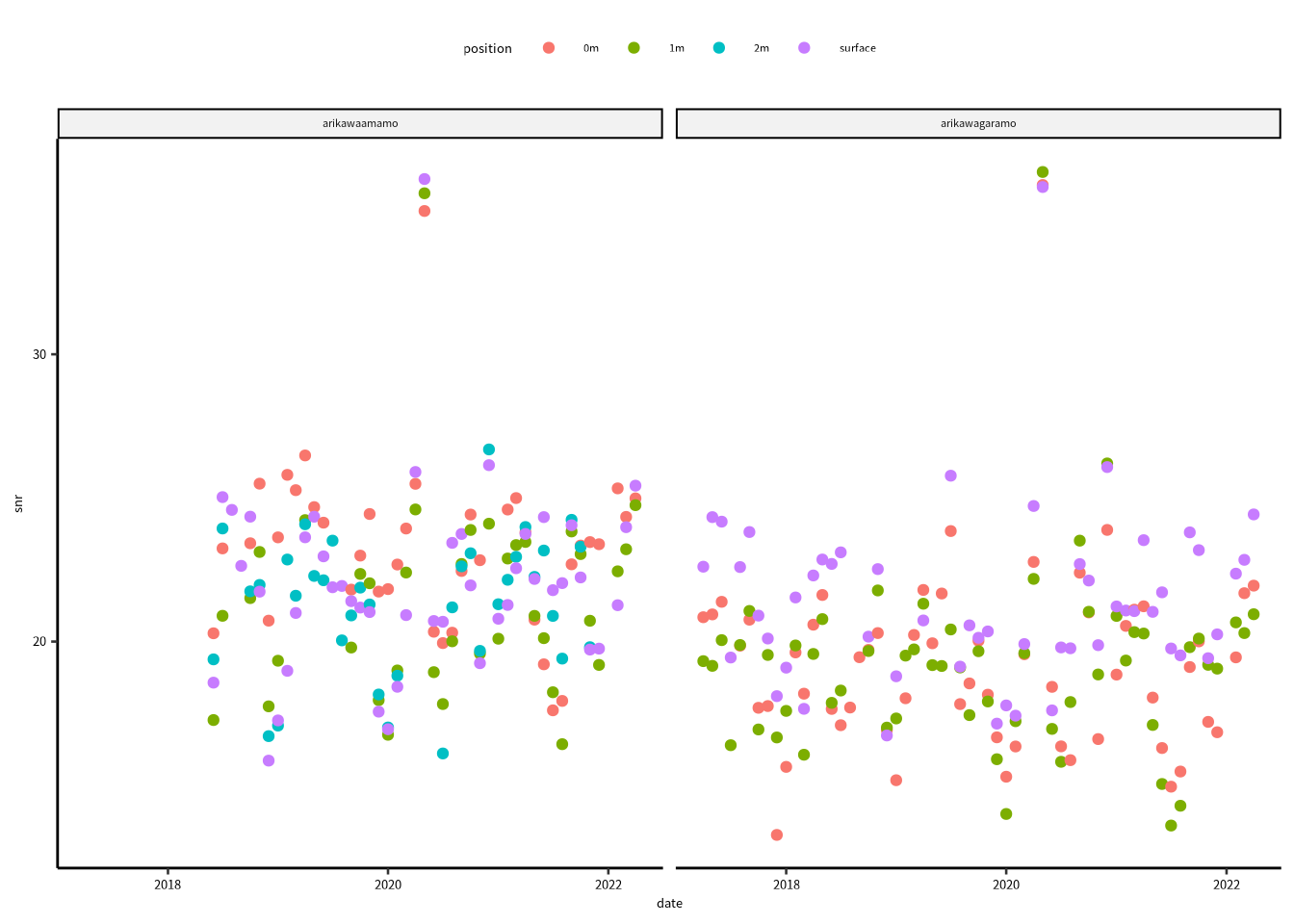

Figure 16.3: SNRは日周期と高周期の比率です。

SNRの傾向を解析して、図に追加します。 locationとposition 間の比較に興味がないので、次のようなモデルを当てはめます。

fit_model = function(df) {
  lm(snr ~ date, data = df)
}

解析の結果

一般線形モデルのF検定の結果、すべてのモデルのP値は 0.05 より大きいですね。

snrdata |> 
  mutate(date = as_date(date)) |> 
  group_nest(location, position) |> 
  mutate(model = map(data, fit_model)) |> 
  mutate(summary = map(model, broom::glance)) |> 
  unnest(summary)
#> # A tibble: 7 × 16
#>   location   position     data model r.squared adj.r.squared
#>   <chr>      <chr>    <list<t> <lis>     <dbl>         <dbl>
#> 1 arikawaam… 0m       [46 × 2] <lm>    0.0131       -0.0128 
#> 2 arikawaam… 1m       [46 × 2] <lm>    0.0210       -0.00623
#> 3 arikawaam… 2m       [41 × 2] <lm>    0.0357        0.00731
#> 4 arikawaam… surface  [46 × 2] <lm>    0.0196       -0.00271
#> 5 arikawaga… 0m       [59 × 2] <lm>    0.00124      -0.0163 
#> 6 arikawaga… 1m       [60 × 2] <lm>    0.00538      -0.0124 
#> 7 arikawaga… surface  [60 × 2] <lm>    0.00406      -0.0151 
#> # … with 10 more variables: sigma <dbl>, statistic <dbl>,
#> #   p.value <dbl>, df <dbl>, logLik <dbl>, AIC <dbl>,
#> #   BIC <dbl>, deviance <dbl>, df.residual <int>,
#> #   nobs <int>

モデル係数の結果は broom パッケージの tidy() 関数で確認できます。

snrdata |> 
  mutate(date = as_date(date)) |> 
  group_nest(location, position) |> 
  mutate(model = map(data, fit_model)) |> 
  mutate(summary = map(model, broom::tidy)) |> 
  unnest(summary) 
#> # A tibble: 14 × 9
#>    location position     data model term  estimate std.error
#>    <chr>    <chr>    <list<t> <lis> <chr>    <dbl>     <dbl>
#>  1 arikawa… 0m       [46 × 2] <lm>  (Int…  3.80e+1 20.8     
#>  2 arikawa… 0m       [46 × 2] <lm>  date  -8.03e-4  0.00113 
#>  3 arikawa… 1m       [46 × 2] <lm>  (Int… -1.19e+0 25.8     
#>  4 arikawa… 1m       [46 × 2] <lm>  date   1.23e-3  0.00140 
#>  5 arikawa… 2m       [41 × 2] <lm>  (Int… -4.24e-1 19.4     
#>  6 arikawa… 2m       [41 × 2] <lm>  date   1.19e-3  0.00106 
#>  7 arikawa… surface  [46 × 2] <lm>  (Int…  2.07e+0 21.4     
#>  8 arikawa… surface  [46 × 2] <lm>  date   1.09e-3  0.00116 
#>  9 arikawa… 0m       [59 × 2] <lm>  (Int…  1.53e+1 14.7     
#> 10 arikawa… 0m       [59 × 2] <lm>  date   2.16e-4  0.000811
#> 11 arikawa… 1m       [60 × 2] <lm>  (Int…  1.12e+1 14.5     
#> 12 arikawa… 1m       [60 × 2] <lm>  date   4.40e-4  0.000799
#> 13 arikawa… surface  [60 × 2] <lm>  (Int…  1.51e+1 13.6     
#> 14 arikawa… surface  [60 × 2] <lm>  date   3.45e-4  0.000750
#> # … with 2 more variables: statistic <dbl>, p.value <dbl>

date はモデル傾きのパラメータです。 arikawaamamo 0m 以外の date 係数は正の値をとっていますが、 Wald’s 検定の結果、すべての P値は 0.05 より大きいです。

帰無仮説検定論によると、0 との統計学的な有意差がなかったので、係数が 0 ではないという仮説は棄却できない。

それにしても、とりあえずデータを図に追加してみよう。

return_fit = function(data, model) {
  nd = data |> expand(date)
  bind_cols(nd, predict(model, newdata = nd, se.fit = TRUE) |> as_tibble()) |> 
    mutate(lower = fit - 1.96*se.fit,
           upper = fit + 1.96*se.fit)
}

snrdata = snrdata |> 
  mutate(date = as_date(date)) |> 
  group_nest(location, position) |> 
  mutate(model = map(data, fit_model)) |>
  mutate(ndata = map2(data,model, return_fit))

ggplot() + 
  geom_line(aes(x = date, y = fit, color = position), data = snrdata |> unnest(ndata)) + 
  geom_point(aes(x = date, y = snr, color = position), data = snrdata |> unnest(data)) + 
  facet_wrap(vars(location))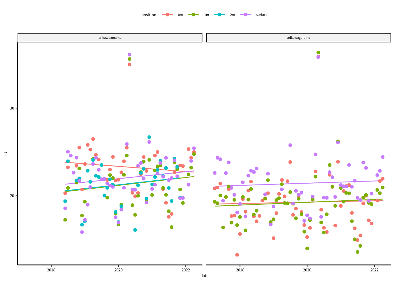

Figure 16.4: SNRの傾向に線形モデルを当てはめたが、線形モデルのF検定に統計学的に有意な結果はありませんでした。

Burrows, Michael T., Robin Harvey, and Linda Robb. “Wave exposure indices from digital coastlines and the prediction of rocky shore community structure.” Marine Ecology Progress Series 353 (2008). https://doi.org/10.3354/meps07284.

Nishihara, Gregory N., Ryuta Terada, and Hiromori Shimabukuro. “Effects of wave energy on the residence times of a fluorescent tracer in the canopy of the intertidal marine macroalgae, Sargassum fusiforme (Phaeophyceae).” Phycological Research 59, no. 1 (2011): 24–33. https://doi.org/10.1111/j.1440-1835.2010.00595.x.

大垣俊一. “開放度測定の地形法.” Argonauta 16 (2009): 25–38. http://wgs.mus-nh.city.osaka.jp/iso/argo/nl16/nl16-25-38.pdf.

15 冗長性分析 (RDA)