14 送風距離 (フェッチ, wind fetch )
海藻は沿岸域における波あたりの強さによって、種数と主構成が変わります16。 波あたりは外界に面した開放性の評価、生物の分布を用いた評価 (biological exposure scale, Burrows et al.、17 地図を用いて方位ごとの対岸距離 (fetch) を求める、観測機器を設置して波あたりの力や波高などの観測が主な評価方法です18。
ここでは、fetch, とくに wind fetch (送風距離)の評価方法を消化します。 波あたりの強さを、生物の分布を用いて評価した場合、波あたりと生物の関係の説明は循環論になります。
送風距離の関数は blasee/fetchR を参考にしました。
14.2 送風距離関数の定義
詳細の原因はわかりませんが、fetchR の関数は国土交通省・国土数値情報
のシェープファイルと合わなかったので、ここで再定義しています。
最大円は calc_circle() で求めます。
map_layer に起点の sf オブジェクトを渡します。
max_dist に最大円の半径を渡します。このときの他には km です。
n_vectors は象限あたりの方位の数です。
calc_circle = function(map_layer, max_dist = 30, n_vectors = 9) {
  # Calculate the fetch limits.
  # max_dist in kilometers
  delta_theta =  360 / (n_vectors * 4)
  theta = seq(0, 360, by = delta_theta)
  n = length(theta)
  theta = theta[-n]
  max_dist = units::set_units(1000*max_dist, "m")
  fetch_circle = st_buffer(map_layer, dist = max_dist, nQuadSegs = n_vectors)
  fetch_limits = st_coordinates(fetch_circle)
  fetch_limits = fetch_limits[-n, ]
  list(fetch_circle = fetch_circle, fetch_limits = as_tibble(fetch_limits[order(theta), ]) )
}
calc_intersection() は起点からフェッチの最大円まで直線を引きます。
最大円内に交差したポリゴンの交差点を特定し、起点に一番近い交差点を返します。
交差点が内場合は、最大円までの距離を返します。
これらの関数は tidyverse や sf が必要です。
calc_intersection = function(fetch_limit, origin, map_layer) {
  X = rbind(st_coordinates(origin), fetch_limit) |> as.matrix()
  fetch_vector = st_linestring(X) |> st_sfc(crs = st_crs(map_layer))
  fetch_intersection = st_intersection(fetch_vector, map_layer) |> st_cast("POINT")
  if(length(fetch_intersection) > 0) {
    intersection_coordinate  = st_coordinates(fetch_intersection) |> as.matrix()
    distance_from_origin = st_distance(origin, fetch_intersection) |> as.vector()
    closest_intersection = min(distance_from_origin)
    n = which(near(distance_from_origin, closest_intersection))
    intersection_coordinate = intersection_coordinate[n,]
  } else {
    intersection_coordinate  = st_point(as.matrix(fetch_limit)) |> st_sfc(crs = st_crs(map_layer))
    distance_from_origin = st_distance(origin, intersection_coordinate) |> as.vector()
    closest_intersection = distance_from_origin
    intersection_coordinate = st_coordinates(intersection_coordinate) |> as.matrix()
  }
  X = matrix(c(st_coordinates(origin), intersection_coordinate[1:2]), ncol = 2, byrow =T)
  fetch_vector = st_linestring(X) |> st_sfc(crs = st_crs(map_layer))
  fetch_length = st_length(fetch_vector)
  fetch_vector |> st_as_sf() |> mutate(length = fetch_length)
}
################################################################################
# Prepare data set #############################################################
# GPS coordinates to determine wind fetcj ######################################
matsushimagps = matrix(rev(c(38.34549669653925, 141.0807915733725)), ncol = 2)
hirotagps     = matrix(rev(c(39.02402594131857, 141.78725806724896)), ncol = 2)
bisegps       = matrix(rev(c(26.704302654710496, 127.85974269102186)), ncol = 2)
arikawagps    = matrix(rev(c(32.98827976845565, 129.11838896005543)), ncol = 2)
# arikawagps    = matrix(rev(c(32.99602966223495, 129.11335509246598)), ncol = 2) # For Fetch calcs
tainouragps   = matrix(rev(c(32.95134175383013, 129.1096027426365)), ncol = 2)
omuragps      = matrix(rev(c(32+52/60+11.9/60/60, 129+58/60+24.5/60/60)), ncol = 2)

gps_info = rbind(matsushimagps, hirotagps, bisegps, arikawagps, tainouragps, omuragps) |>
  as_tibble() |>
  mutate(name = c("matsushimagps", "hirotagps", "bisegps", "arikawagps", "tainouragps", "omuragps")) |>
  mutate(label = str_to_sentence(str_remove(name, pattern = "(gps)"))) |>
  rename(long = V1, lat = V2)

gps_info = gps_info |>
  mutate(label2 = str_to_sentence(label)) |>
  mutate(label2 = str_glue("{label2} {ifelse(str_detect(label2, 'Bise'), 'Point', 'Bay')}"))

# Prepare the Coordinate Reference System to be EPSG:4326 (Which is WGS 84)
# See st_crs(4326) for details
gps_info = gps_info |> select(long, lat, name) |> st_as_sf(coords = c("long", "lat"), crs = 4326, agr = "constant")

# Load the map shape files #####################################################
# The map uses the ITRF94 system (st_crs(map_poly))
# gsi_low = read_sf("~/Lab_Data/Japan_map_data/GSI/coastl_jpn.shp")
# gsi_low = read_sf("~/Lab_Data/Japan_map_data/GADM_old/JPN_adm1.shp")
map_poly = read_sf("~/Lab_Data/Japan_map_data/GSI/polbnda_jpn.shp")
map_poly = map_poly |> select(nam, geometry)

# Convert the CRS to EPSG:2450 #################################################
map_poly = st_transform(map_poly, st_crs(2450))
gps_info  = st_transform(gps_info, st_crs(2450))

################################################################################
# Do the analysis one location at a time. ######################################
ptsize = 1
max_dist = 10 # In km
n_vectors = 3*9 # The number of vectors in every quadrant.

location = "Hirota Bay"
polygon_layer = subset(map_poly, str_detect(nam, "Iwate")) |> st_union()
site_layer    = subset(gps_info, str_detect(name, "hiro"))
fetch_limits = calc_circle(site_layer, max_dist = max_dist, n_vectors = n_vectors)
fout = fetch_limits$fetch_limits |>
  mutate(fe  = map2(X,Y,function(x,y) cbind(x,y))) |>
  mutate(geometry = map(fe, calc_intersection, origin = site_layer, map_layer = polygon_layer))
fout = fout |> select(geometry) |>  unnest(geometry) |> st_as_sf()
temp_layer = st_crop(polygon_layer, st_bbox(fetch_limits$fetch_circle))
mean_fetch = fout |> pull(length) |> mean() |> as.numeric()
sd_fetch = fout |> pull(length) |> sd() |> as.numeric()
max_fetch = fout |> pull(length) |> as.numeric()
man_n = sum(near(max_fetch, max_dist * 1000))
tot_n = length(max_fetch)

p1 = ggplot() +
  geom_sf(data = temp_layer, color = NA) +
  geom_sf(data = fout) +
  geom_sf(data = site_layer, color = "red", size = ptsize) +
  labs(title = str_glue("The mean ± sd fetch for {location} is {format(mean_fetch, digits = 4)} ± {format(sd_fetch, digits = 4)} m."),
       subtitle = str_glue("{man_n} out of {tot_n} vectors were at the upper limit."))

location = "Matsushima Bay"
polygon_layer = subset(map_poly, str_detect(nam, "Miyag")) |> st_union()
site_layer    = subset(gps_info, str_detect(name, "matsu"))
fetch_limits = calc_circle(site_layer, max_dist = max_dist, n_vectors = n_vectors)
fout = fetch_limits$fetch_limits |> as_tibble() |>
  mutate(fe  = map2(X,Y,function(x,y) cbind(x,y))) |>
  mutate(geometry = map(fe, calc_intersection, origin = site_layer, map_layer = polygon_layer))
fout = fout |> select(geometry) |>  unnest(geometry) |> st_as_sf()
temp_layer = st_crop(polygon_layer, st_bbox(fetch_limits$fetch_circle))
mean_fetch = fout |> pull(length) |> mean() |> as.numeric()
sd_fetch = fout |> pull(length) |> sd() |> as.numeric()
max_fetch = fout |> pull(length) |> as.numeric()
man_n = sum(near(max_fetch, max_dist * 1000))
tot_n = length(max_fetch)

p2 = ggplot() +
  geom_sf(data = temp_layer, color = NA) +
  geom_sf(data = fout) +
  geom_sf(data = site_layer, color = "red", size = ptsize) +
  labs(title = str_glue("The mean ± sd fetch for {location} is {format(mean_fetch, digits = 4)} ± {format(sd_fetch, digits = 4)} m."),
       subtitle = str_glue("{man_n} out of {tot_n} vectors were at the upper limit."))

location = "Bise Point"
polygon_layer = subset(map_poly, str_detect(nam, "Okinawa")) |> st_union()
site_layer    = subset(gps_info, str_detect(name, "bise"))
fetch_limits = calc_circle(site_layer, max_dist = max_dist, n_vectors = n_vectors)
fout = fetch_limits$fetch_limits |> as_tibble() |>
  mutate(fe  = map2(X,Y,function(x,y) cbind(x,y))) |>
  mutate(geometry = map(fe, calc_intersection, origin = site_layer, map_layer = polygon_layer))
fout = fout |> select(geometry) |>  unnest(geometry) |> st_as_sf()
temp_layer = st_crop(polygon_layer, st_bbox(fetch_limits$fetch_circle))
mean_fetch = fout |> pull(length) |> mean() |> as.numeric()
sd_fetch = fout |> pull(length) |> sd() |> as.numeric()
max_fetch = fout |> pull(length) |> as.numeric()
man_n = sum(near(max_fetch, max_dist * 1000))
tot_n = length(max_fetch)

p3 = ggplot() +
  geom_sf(data = temp_layer, color = NA) +
  geom_sf(data = fout) +
  geom_sf(data = site_layer, color = "red", size = ptsize) +
  labs(title = str_glue("The mean ± sd fetch for {location} is {format(mean_fetch, digits = 4)} ± {format(sd_fetch, digits = 4)} m."),
       subtitle = str_glue("{man_n} out of {tot_n} vectors were at the upper limit."))

location = "Omura Bay"
polygon_layer = subset(map_poly, str_detect(nam, "Nagasaki")) |> st_union()
site_layer    = subset(gps_info, str_detect(name, "omura"))
fetch_limits = calc_circle(site_layer, max_dist = max_dist, n_vectors = n_vectors)
fout = fetch_limits$fetch_limits |> as_tibble() |>
  mutate(fe  = map2(X,Y,function(x,y) cbind(x,y))) |>
  mutate(geometry = map(fe, calc_intersection, origin = site_layer, map_layer = polygon_layer))
fout = fout |> select(geometry) |>  unnest(geometry) |> st_as_sf()
temp_layer = st_crop(polygon_layer, st_bbox(fetch_limits$fetch_circle))
mean_fetch = fout |> pull(length) |> mean() |> as.numeric()
sd_fetch = fout |> pull(length) |> sd() |> as.numeric()
max_fetch = fout |> pull(length) |> as.numeric()
man_n = sum(near(max_fetch, max_dist * 1000))
tot_n = length(max_fetch)

p4 = ggplot() +
  geom_sf(data = temp_layer, color = NA) +
  geom_sf(data = fout) +
  geom_sf(data = site_layer, color = "red", size = ptsize) +
  labs(title = str_glue("The mean ± sd fetch for {location} is {format(mean_fetch, digits = 4)} ± {format(sd_fetch, digits = 4)} m."),
       subtitle = str_glue("{man_n} out of {tot_n} vectors were at the upper limit."))

location = "Arikawa Bay"
polygon_layer = subset(map_poly, str_detect(nam, "Nagasaki")) |> st_union()
site_layer    = subset(gps_info, str_detect(name, "arik"))
fetch_limits = calc_circle(site_layer, max_dist = max_dist, n_vectors = n_vectors)
fout = fetch_limits$fetch_limits |> as_tibble() |>
  mutate(fe  = map2(X,Y,function(x,y) cbind(x,y))) |>
  mutate(geometry = map(fe, calc_intersection, origin = site_layer, map_layer = polygon_layer))
fout = fout |> select(geometry) |>  unnest(geometry) |> st_as_sf()
temp_layer = st_crop(polygon_layer, st_bbox(fetch_limits$fetch_circle))
mean_fetch = fout |> pull(length) |> mean() |> as.numeric()
sd_fetch = fout |> pull(length) |> sd() |> as.numeric()

max_fetch = fout |> pull(length) |> as.numeric()
man_n = sum(near(max_fetch, max_dist * 1000))
tot_n = length(max_fetch)

p5 = ggplot() +
  geom_sf(data = temp_layer, color = NA) +
  geom_sf(data = fout) +
  geom_sf(data = site_layer, color = "red", size = ptsize) +
  labs(title = str_glue("The mean ± sd fetch for {location} is {format(mean_fetch, digits = 4)} ± {format(sd_fetch, digits = 4)} m."),
       subtitle = str_glue("{man_n} out of {tot_n} vectors were at the upper limit."))

location = "Tainoura Bay"
polygon_layer = subset(map_poly, str_detect(nam, "Nagasaki")) |> st_union()
site_layer    = subset(gps_info, str_detect(name, "tain"))
fetch_limits = calc_circle(site_layer, max_dist = max_dist, n_vectors = n_vectors)
fout = fetch_limits$fetch_limits |> as_tibble() |>
  mutate(fe  = map2(X,Y,function(x,y) cbind(x,y))) |>
  mutate(geometry = map(fe, calc_intersection, origin = site_layer, map_layer = polygon_layer))
fout = fout |> select(geometry) |>  unnest(geometry) |> st_as_sf()
temp_layer = st_crop(polygon_layer, st_bbox(fetch_limits$fetch_circle))
mean_fetch = fout |> pull(length) |> mean() |> as.numeric()
sd_fetch = fout |> pull(length) |> sd() |> as.numeric()

max_fetch = fout |> pull(length) |> as.numeric()
man_n = sum(near(max_fetch, max_dist * 1000))
tot_n = length(max_fetch)

p6 = ggplot() +
  geom_sf(data = temp_layer, color = NA) +
  geom_sf(data = fout) +
  geom_sf(data = site_layer, color = "red", size = ptsize) +
  labs(title = str_glue("The mean ± sd fetch for {location} is {format(mean_fetch, digits = 4)} ± {format(sd_fetch, digits = 4)} m."),
       subtitle = str_glue("{man_n} out of {tot_n} vectors were at the upper limit."))
(p1 + p2 + p3) / (p4 + p5 + p6)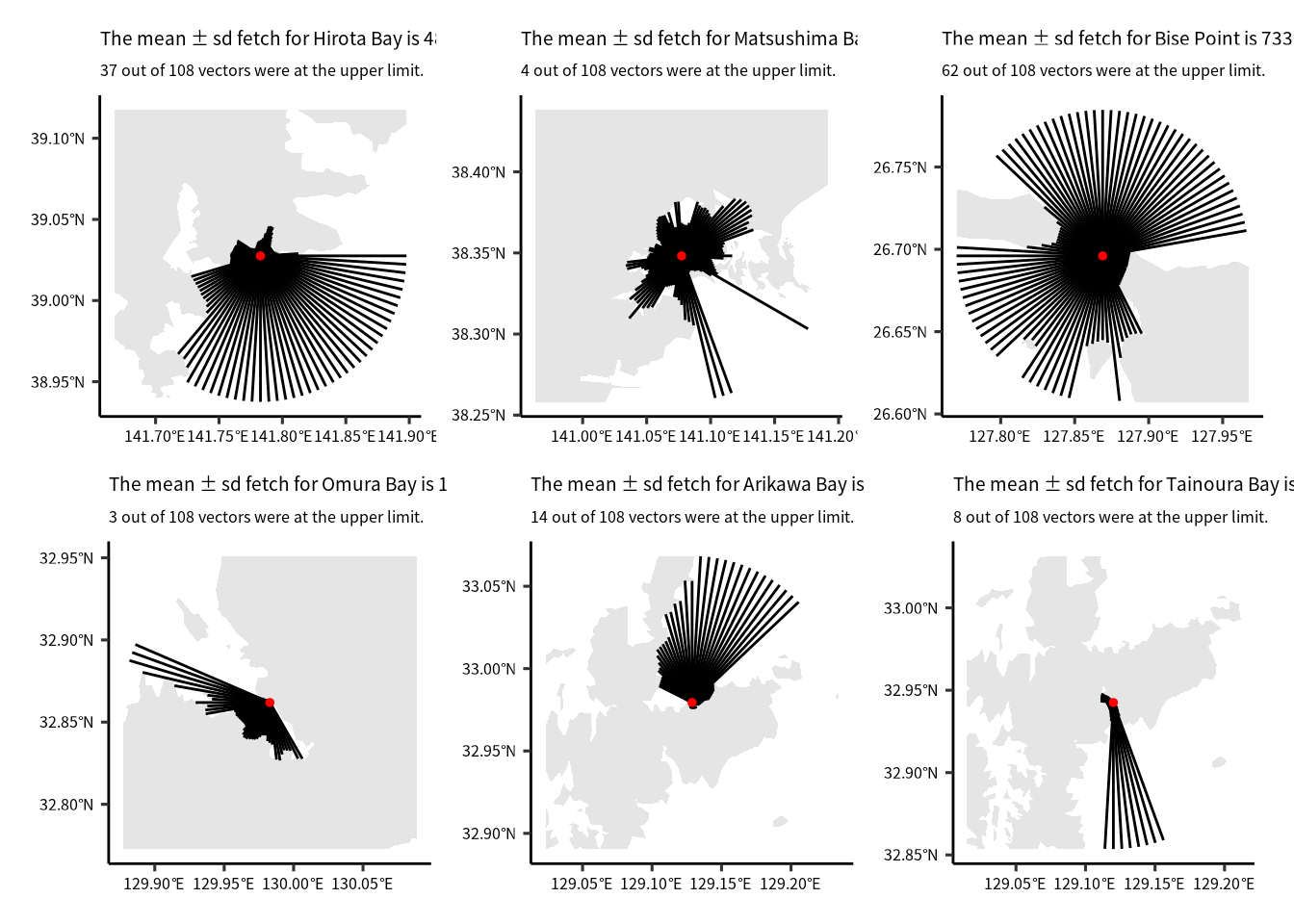
pdfname = "~/Downloads/Determine_fetch.pdf"
pngname = str_replace(pdfname, "pdf", "png")
ggsave(pdfname, width = 5*80, height = 4*80, units = "mm")
img = image_read(pdfname, density = 300)
img |> image_write(pngname, format = "png")
Gregory N. Nishihara, Ryuta Terada, and Hiromori Shimabukuro, “Effects of wave energy on the residence times of a fluorescent tracer in the canopy of the intertidal marine macroalgae, Sargassum fusiforme (Phaeophyceae),” Phycological Research 59, no. 1 (2011): 24–33, https://doi.org/10.1111/j.1440-1835.2010.00595.x.↩︎
Michael T. Burrows, Robin Harvey, and Linda Robb, “Wave exposure indices from digital coastlines and the prediction of rocky shore community structure,” Marine Ecology Progress Series 353 (2008), https://doi.org/10.3354/meps07284.↩︎
大垣俊一, “開放度測定の地形法,” Argonauta 16 (2009): 25–38, http://wgs.mus-nh.city.osaka.jp/iso/argo/nl16/nl16-25-38.pdf.↩︎