有川湾の藻場で観測した魚類

パッケージの読み込み

library(tidyverse)

── Attaching core tidyverse packages ──────────────────────── tidyverse 2.0.0 ──
✔ dplyr     1.1.4     ✔ readr     2.1.5
✔ forcats   1.0.0     ✔ stringr   1.5.1
✔ ggplot2   3.5.1     ✔ tibble    3.2.1
✔ lubridate 1.9.3     ✔ tidyr     1.3.1
✔ purrr     1.0.2     
── Conflicts ────────────────────────────────────────── tidyverse_conflicts() ──
✖ purrr::%||%()   masks base::%||%()
✖ dplyr::filter() masks stats::filter()
✖ dplyr::lag()    masks stats::lag()
ℹ Use the conflicted package (<http://conflicted.r-lib.org/>) to force all conflicts to become errors

データの読み込み

データはこちらからダウンロードできます。

fish_data - fish_data.csv

filename = "fish_data - fish_data.csv"
fish = read_csv(filename)

読み込んだデータの中身を確認しましょう。

fish

線データの記述統計量は次の通りです。 drop_na() は欠損値を除外する関数です。 arrange() はデータを並び替える関数です。 NA は欠損値を表します。

fish |> 
  drop_na() |> 
  group_by(Species) |> 
  summarise(n = n(), 
            mean = mean(Count),
            sd = sd(Count),
            min = min(Count),
            max = max(Count)) |> 
  arrange(desc(n))

データを抽出する

今回は，種ごとにデータを抽出してから解析をします。 まずは，データに含まれる種を確認します。

fish |> pull(Species) |> unique()

 [1] "メジナ"       "アイゴ"       "イスズミ"     "キタマクラ"   "タカノハダイ"
 [6] "ニザダイ"     "ブダイ"       "カワハギ"     "ボラ"         "アオブダイ"  
[11] "ハコフグ"     "カワハギ　"  

では，メジナ，アイゴ，イスズミのデータを抽出してみましょう。

mejina =  fish |> filter(str_detect(Species, "メジナ"))
aigo =    fish |> filter(str_detect(Species, "アイゴ"))
isuzumi = fish |> filter(str_detect(Species, "イスズミ"))

dset_ai = bind_rows(aigo, isuzumi)
dset_am = bind_rows(aigo, mejina)
dset_im = bind_rows(isuzumi, mejina)

データの可視化

ggplot() + 
geom_boxplot(
  aes(x = Species, 
      y = Count, 
      color = Species), data = dset_ai)

Figure 1: アイゴとイスズミの数の比較

ggplot() + 
geom_boxplot(
  aes(x = Species, 
      y = Count, 
      color = Species), data = dset_am)

Warning: Removed 1 row containing non-finite outside the scale range
(`stat_boxplot()`).

Figure 2: アイゴとメジナの数の比較

ggplot() + 
geom_boxplot(
  aes(x = Species, 
      y = Count, 
      color = Species), data = dset_im)

Warning: Removed 1 row containing non-finite outside the scale range
(`stat_boxplot()`).

Figure 3: イスズミとメジナの数の比較

t検定

Note

仮説検定論のとき，有意水準 (\alpha) を決める必要があります。 一般的には \alpha = 0.05 が使われますが， 研究分野や研究目的によっては \alpha = 0.01 や \alpha = 0.10 が使われることもあります。

アイゴとイスズミの数の比較

• 帰無仮説 (H_0)：アイゴとイスズミの個体数に違いがない
• 対立仮設 (H_A)：アイゴとイスズミの個体数に違いがある

t.test(Count ~ Species, data = dset_ai)

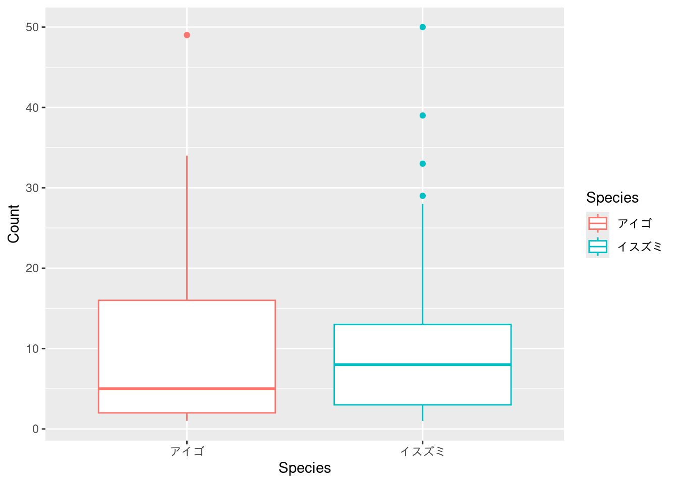
    Welch Two Sample t-test

data:  Count by Species
t = 0.22226, df = 94.657, p-value = 0.8246
alternative hypothesis: true difference in means between group アイゴ and group イスズミ is not equal to 0
95 percent confidence interval:
 -3.525656  4.414545
sample estimates:
  mean in group アイゴ mean in group イスズミ 
             10.428571               9.984127 

アイゴとイスズミの個体数を比較したとき， t値 = 0.2223 でした。 このときの 自由度は 94.66 であり， p値 = 0.8246 でした。 P値は有意水準より高かったため，帰無仮説を棄却できませんでした。

アイゴとメジナの数の比較

• 帰無仮説 (H_0)：アイゴとメジナの個体数に違いがない
• 対立仮設 (H_A)：アイゴとメジナの個体数に違いがある

t.test(Count ~ Species, data = dset_am)

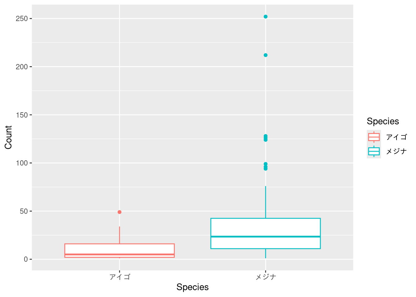
    Welch Two Sample t-test

data:  Count by Species
t = -5.045, df = 89.48, p-value = 2.361e-06
alternative hypothesis: true difference in means between group アイゴ and group メジナ is not equal to 0
95 percent confidence interval:
 -37.03593 -16.10692
sample estimates:
mean in group アイゴ mean in group メジナ 
            10.42857             37.00000 

アイゴとメジナの個体数を比較したとき， t値 = -5.0450 でした。 このときの 自由度は 89.48 であり， p値 = 2.3607e-06 でした。 P値は有意水準より低かったため，帰無仮説を棄却できました。

イスズミとメジナの数の比較

• 帰無仮説 (H_0)：イスズミとメジナの個体数に違いがない
• 対立仮設 (H_A)：イスズミとメジナの個体数に違いがある

t.test(Count ~ Species, data = dset_im)

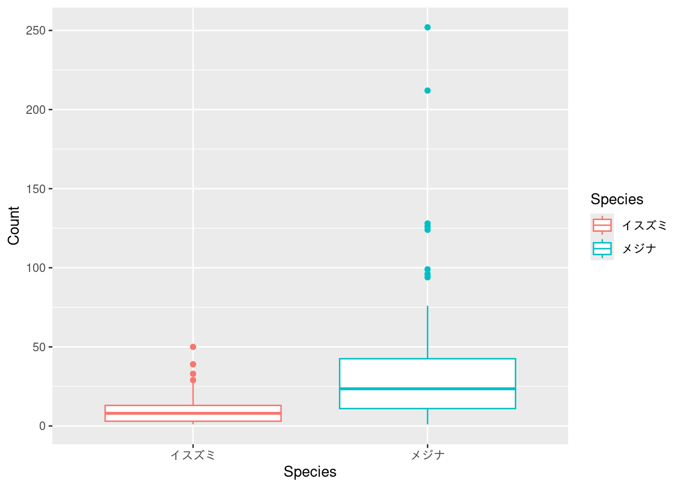
    Welch Two Sample t-test

data:  Count by Species
t = -5.233, df = 83.577, p-value = 1.218e-06
alternative hypothesis: true difference in means between group イスズミ and group メジナ is not equal to 0
95 percent confidence interval:
 -37.28307 -16.74868
sample estimates:
mean in group イスズミ   mean in group メジナ 
              9.984127              37.000000 

イスズミとメジナの個体数を比較したとき， t値 = -5.2330 でした。 このときの 自由度は 83.58 であり， p値 = 1.2179e-06 でした。 P値は有意水準より低かったため，帰無仮説を棄却できました。