[1] "en_US.UTF-8"開放型溶存酸素法
フォントの準備
ここではフォントと図のテーマを設定する。
Code
# R 環境の準備 #############################################
font_add_google("Noto Sans","notosans")
font_add_google("Noto Sans JP","notosans-jp")

# ggplot のデフォルト設定
theme_pubr(base_size = 24,
           base_family = "notosans") |> theme_set()
showtext_auto()
関数を定義する
Code
calculate_dawn_dusk = possibly(function(datetime, gpscoord) {
  # 光のデータが十分じゃない時、日中の長さを求められないので、
  # 薄暮と薄明は crepuscule で求める
  # suntools のパッケージが必要
  # solarDep = 6 is civil twilight (市民薄明)
  # solarDep = 18 is astronomical twilight (天文薄明)
  tz(datetime) = "Japan"
  dawn = suntools::crepuscule(
    gpscoord,
    datetime,
    solarDep = 6,
    direction = "dawn",
    POSIXct = T
  )[, 2]
  dusk = suntools::crepuscule(
    gpscoord,
    datetime,
    solarDep = 6,
    direction = "dusk",
    POSIXct = T
  )[, 2]
  tz(dawn) = "UCT"
  tz(dusk) = "UCT"
  interval(dawn, dusk)
}, otherwise = NULL)

calculate_rate =
  possibly(function(dset, k = 48) {
    # 酸素変動速度の計算
    require(mgcv)
    require(gratia)
    newton = list(maxNstep = 10, maxHalf = 50)
    gcontrol = gam.control(maxit = 500, newton = newton)
    out = gam(mgl ~ s(H, k = k, bs = "cs"),
              data = dset,
              family = gaussian(link = "identity"),
              control = gcontrol
    )
    tmp = dset |> select(H, mgl)
    fitted = add_fitted(tmp, out, value = "fitted") |>
      pull(fitted)
    rate = derivatives(out,
                       data = tmp,
                       type = "central") |>
      pull(.derivative)
    dset |> mutate(fitted, rate)
  }, otherwise = NULL)

masstransfer =
  possibly(function(windspeed,
                    temperature,
                    salinity,
                    oxygen,
                    pressure,
                    height = 1) {
    # 大気と海面における酸素の輸送の計算
    # marelac パッケージが必要
    # height は m, salinity は PSU
    calc_k600 = function(windspeed, height) {
      # Crusius and Wanninkhof 2003 L&O 48
      cf = 1 + sqrt(1.3e-3) / 0.4 * (log(10 / height))
      U10 = cf * windspeed # m/s
      0.228 * U10 ^ 2.2 + 0.168 # cm/h
    }
    k600 = calc_k600(windspeed, height)
    SCoxygen = marelac::gas_schmidt(temperature, species = "O2")
    a = ifelse(windspeed < 3, 2 / 3, 1 / 2)
    kx = k600 * (600 / SCoxygen) ^ a # cm / h
    # pressure は hecto-pascal
    o2sat = marelac::gas_satconc(salinity, temperature,
                                 pressure / 1000,
                                 species = "O2") # mmol / m3
    o2sat = o2sat * 32 / 1000
    kx / 100 * (o2sat - oxygen) # g / m2 / h
  }, otherwise = NULL)
\begin{aligned} U_{10} &= U_h\left[1 + \frac{{C_{d10}}^{0.5}}{\kappa} ln\left(\frac{10}{h}\right)\right]\\ C_{d10} &= 1.3\times 10^{-3} \\ \kappa &= 0.4\\ k_{600} &= 0.228 {U_{10}}^{2.2}+ 0.168\\ k_t &= k_{600} \left(\frac{600}{Sc({\text{oxygen}})}\right)^a\\ a &= \begin{cases} \frac{2}{3}, & \text{if } w<3 \\ \frac{1}{2}, & \text{if } w>=3 \\ \end{cases}\\ F_{tspw} &= 0.1\times k_t \left(O_{2sat} - O_2\right)\\ \end{aligned} \tag{1}
Equation 1 は次の論文を参考に: Crucis & Wanninkhof 2003 Limnol & Oceanogr 48(3): 1010 - 1017 (https://doi.org/10.4319/lo.2003.48.3.1010). 海面における酸素のフラックスは t 水温、s 塩分, p 気圧, w 風速によって影響される。 O_{2sat}は海水面における溶存酸素飽和能動です。 O_2はデータロガーで観測した溶存酸素濃度です。 Sc(\text{oxygen}) は酸素のシュミット数です。
データの紹介
Code
datasetCode
p1 = ggplot(dataset) +
  geom_line(aes(x = datetime,
                y = mgl))
p2 = ggplot(dataset) +
  geom_line(aes(x = datetime,
                y = temperature))
p3 = ggplot(dataset) +
  geom_line(aes(x = datetime,
                y = wind))
p4 = ggplot(dataset) +
  geom_line(aes(x = datetime,
                y = hpa))
p5 = ggplot(dataset) +
  geom_line(aes(x = datetime,
                y = depth))

p1 + p2 + p3 + p4 + p5 + plot_layout(ncol = 1)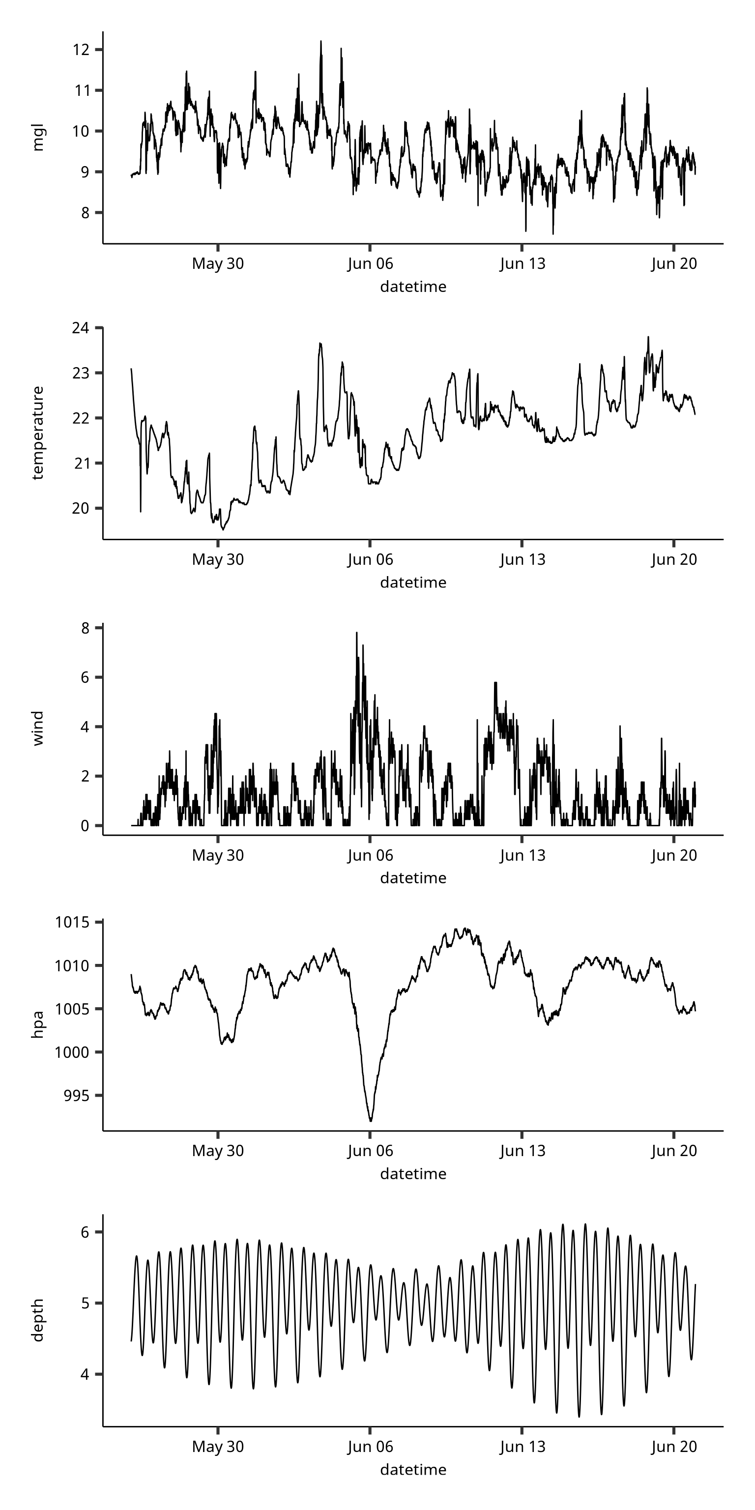
酸素変動速度の求め方
Code
dset = dataset |>
  group_nest(date) |>
  slice(10) |>
  unnest(data)
溶存酸素濃度のデータには一般化加法モデル(GAM, Generalized Additive Model) (Equation 2) を当てはめます。
y = f_{24}(x) \tag{2}
y は溶存酸素濃度、x は時間, f_{24}() は3次スプラインです。 データの時間情報は時刻表示から時に変えます。 24 はスプラインの基底の数です。
Code
calc_hours = function(x) {
  hour(x) + minute(x) / 60 + second(x) / 3600
}
dset = dset |>
mutate(H = calc_hours(datetime), .after = datetime)データの準備ができたら、Equation 2 を当てはめます。 当てはめたモデルから接線を求めて、酸素濃度の変動速度を求めます。
Code
m1 = gam(mgl ~ s(H, k = 24, bs = "cr"), data = dset)
pdata = dset |> add_fitted(model = m1, value = "fit")
rate = derivatives(m1, data = pdata, type = "central") |>
  pull(.derivative)
pdata = pdata |>
  mutate(rate = rate * depth) |>
  mutate(deltat = 24 / n()) |>
  mutate(mt = masstransfer(wind, temperature, 35, mgl, hpa, 1))
当てはめたデータ (Dissolve oxygen) と計算した溶存酸素濃度の変動速度 (Oxygen exchange rate), 海水面における溶存酸素濃度のフラックス (Mass transfer rate), 最終的に求めた生態系純一次生産量 (NEP) は Figure 1 に示した。
Code
ylab1 = "Dissolved oxygen (g O<sub>2</sub> m<sup>-3</sup>)"
ylab2 = "Oxygen exchange rate (g O<sub>2</sub> m<sup>-2</sup> h<sup>-1</sup>)"
ylab3 = "Mass transfer rate (g O<sub>2</sub> m<sup>-2</sup> h<sup>-1</sup>)"
ylab4 = "NEP (g O<sub>2</sub> m<sup>-2</sup> h<sup>-1</sup>)"

p1 = ggplot() +
  geom_point(aes(x = H, y = mgl), data = dset,
             alpha = 0.5, shape = 21, stroke = NA,
             bg = "navy", size = 3) +
  geom_line(aes(x = H, y = fit), data = pdata,
            color = "navy", linewidth = 1) +
  scale_x_continuous("Hour", breaks = seq(0, 24, by = 6),
                     limits = c(0,24)) +
  scale_y_continuous(ylab1,
                     limits = c(9, 13)) +
  theme(axis.title.y.left = element_markdown(),
        axis.title.y.right = element_markdown())
p2 = ggplot() +
  geom_line(aes(x = H, y = rate), data = pdata,
            color = "navy", linewidth = 1) +
  scale_x_continuous("Hour", breaks = seq(0, 24, by = 6),
                     limits = c(0,24)) +
  scale_y_continuous(ylab2,
                     limits = c(-5, 5)) +
  theme(axis.title.y.left = element_markdown(),
        axis.title.y.right = element_markdown())
p3 = ggplot() +
  geom_line(aes(x = H, y = mt), data = pdata,
            color = "navy", linewidth = 1) +
  scale_x_continuous("Hour", breaks = seq(0, 24, by = 6),
                     limits = c(0,24)) +
  scale_y_continuous(ylab3, limits = c(-0.15, 0)) +
  theme(axis.title.y.left = element_markdown(),
        axis.title.y.right = element_markdown())
p4 = ggplot() +
  geom_line(aes(x = H, y = rate - mt), data = pdata,
            color = "navy", linewidth = 1) +
  scale_x_continuous("Hour", breaks = seq(0, 24, by = 6),
                     limits = c(0,24)) +
  scale_y_continuous(ylab4, limits = c(-5, 5)) +
  theme(axis.title.y.left = element_markdown(),
        axis.title.y.right = element_markdown())
p1 + p2 + p3 + p4 + plot_layout(ncol = 1)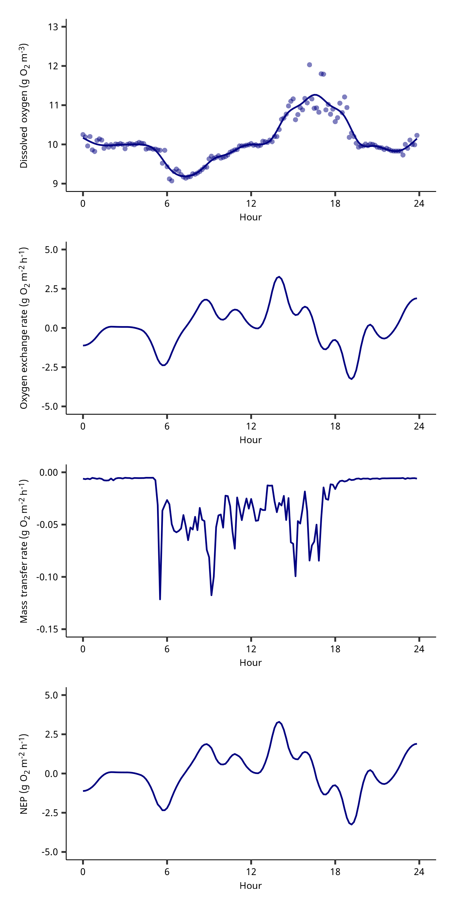
Figure 1 の NEP を積算することで、一日あたりのNEPを求められます (Equation 3)。 これは Sato et al. 2022 (https://doi.org/10.3389/fmars.2022.861932) と同じ方法です。
O_{2,\text{day}} = \sum (\text{Rate}\Delta t) \tag{3}
Code
npp = pdata |>
  mutate(nep = rate - mt) |>
  summarise(nep = sum(nep)) |>
  pull(nep)
一日あたりの蓄積量はは 11.05 g O2 m-2 d-1 でした。 領域の境界がわからないフィールドの場合は、この結果は純一次生産量します。
紹介したデータの結果
Code
fitdataset = function(dset) {
m1 = gam(mgl ~ s(H, k = 24, bs = "cr"), data = dset)
pdata = dset |> add_fitted(model = m1, value = "fit")
rate = derivatives(m1, data = pdata, type = "central") |>
pull(.derivative)
pdata = pdata |>
mutate(rate = rate * depth) |>
mutate(deltat = 24 / n()) |>
mutate(mt = masstransfer(wind, temperature, 35, mgl, hpa, 1))
pdata
}
dataset = dataset |>
group_nest(date) |>
mutate(data2 = map(data, fitdataset))
dataset2 = dataset |>
unnest(data2) |>
mutate(nep = rate - mt) |>
group_by(date) |>
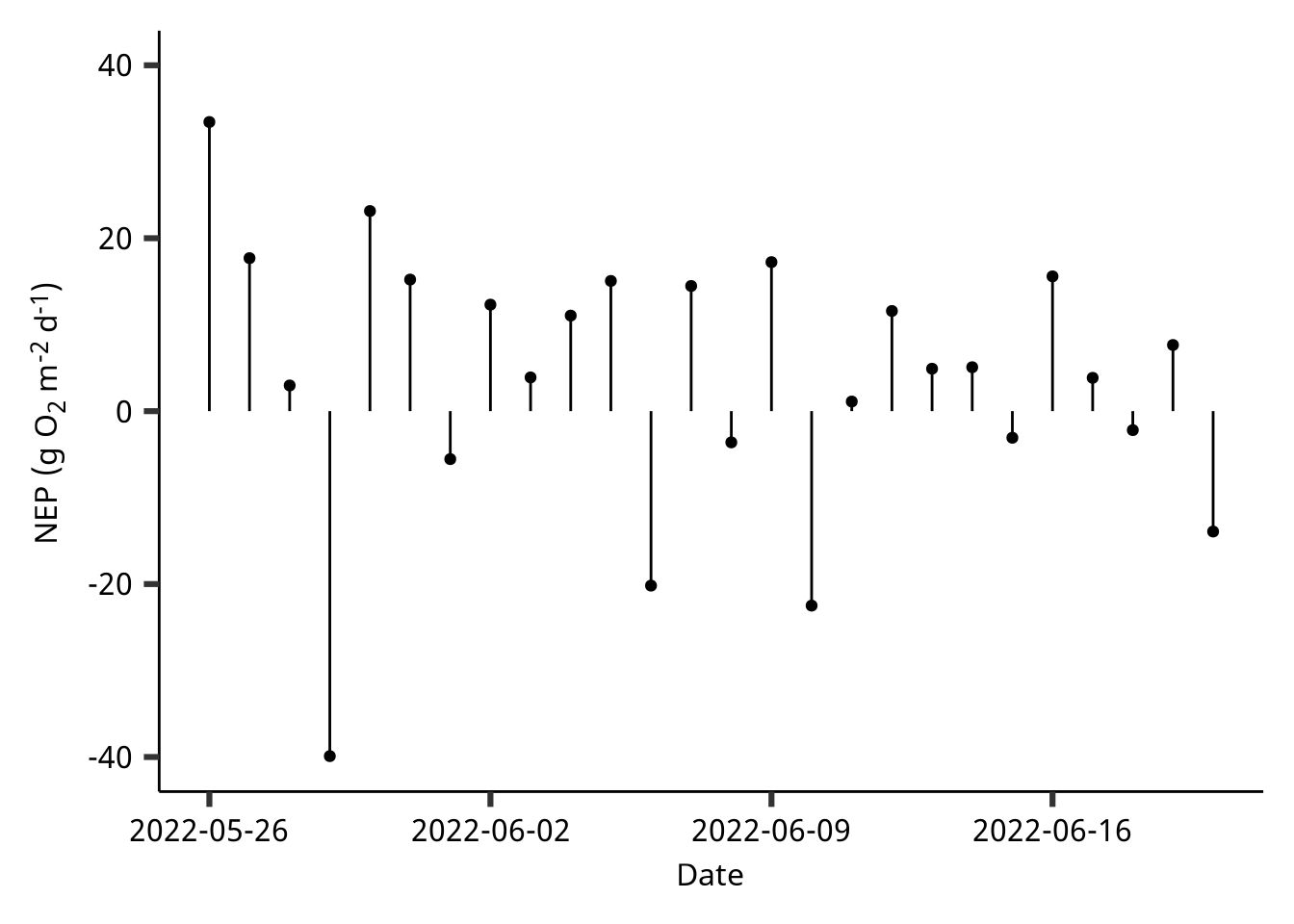
summarise(nep = sum(nep))Code
ylabel = "NEP (g O<sub>2</sub> m<sup>-2</sup> d<sup>-1</sup>)"

ggplot(dataset2) +
  geom_point(aes(x = date, y = nep)) +
  geom_segment(aes(x = date, xend = date,
                   y = 0, yend = nep)) +
  scale_y_continuous(ylabel,
                     limits = c(-40, 40)) +
  scale_x_date("Date",
               breaks = "7 days") +
  theme(axis.title.y = element_markdown())